Stanford CS229M - Lecture 2: Asymptotic analysis, uniform convergence, Hoeffding inequality

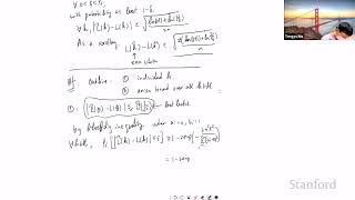
okay cool let's get started so uh uh okay it's kind of complicated right like a it's kind of amazing right like this technology is so Advanced so that you can do all of these things together but uh I still have to do them one by one like I have like 10 action items maybe more than 10. I need to also connects with Wi-Fi that's uh that's actually something I have to do um okay so but oh let's let's get started oh I need to have my notes so what we're going to do today is that we're going to continue with the asymptotics last time a little bit for like a about like 15 to 20 minutes um this is just to wrap up what we have discussed um and as I said this uh first lecture is always kind of like a little bit tricky to for me to teach it because um the tools there you know if you want to make it formal it requires some kind of backgrounds um and if you don't want to make it formal sometimes there is a little bit confusion so um from from the this lecture the second half of this lecture I think we are going to talk about um things that require less background in some sense um and it's more self-content okay so the plan is that asymptotics and then um the so-called uniform convergence I'll Define what it is and uniform convergence will be the main focus for the first few weeks of the lecture okay so let's start by reviewing what we have done last time so what we have the last time was this theorem where we showed that um um if you assume consistency which is something that is kind of like we basically just assume without much justification you know um it's not always true and it also depends on the problem uh the consistency basically means that set a hat will converge to Theta star we call that hat is the ERM the empirical risk minimizer and Theta star is the minimizer of the population risk so you care about recovering through the star or recovering something as good as the star and we also assume a bunch of other things like for example The Hyphen is full rank and also some regulatory conditions which I didn't even Define um exactly for example this requires something like some of the virus it's financed so you can apply the serums and then under this assumptions we have that actually it's kind of challenging for me because this Podium after I read it it becomes unstable it's kind of like I feel like I'm writing where I'm on a boat um but it's probably good for me to practice my kind of like what is this called like I would be better with some of the sports I guess after you do this anyway okay so uh so I guess we have discussed that you know that's the distribution you know the order of the difference between Cedar height and sales star the order is on the order of one over square root n and formally write it like this you scale backwards in and you know that it's on the other four and you also know something about the laws you know that the excess risk L to the Hat minus l0 star is on the on the order of one over n and if you formally write it you are going to scale by n and then you say it's on all the constants and also you know that the distribution of theta hat minus the star this is converging to a gaussian distribution which means zero and some covariance and this covariance is kind of complicated but let me write it um something like this this is just reviewing what we have written last time and four we also know the the distribution of the excess risk this is a distribution of a scalar because the accessories is a scalar it will scale it by n then you know the distribution is converging to the distribution of this random variable and this random variable as is a gaussian random variable with covariance means zero and covariance something like above but not exactly you don't have to remember exactly what the covariance here is because you know I don't even remember them um if I don't read my notes these are you know there are some intuitions about this which I'm going to discuss but generally this is just uh was something you got from derivations so so last time we have kind of like roughly justify the number one number two and today I'm going to again give a relatively heuristic approve for three and four just very quick so that we can wrap up this um um so I guess just to very quickly review what we have done last time so the key idea to kind of like derive all of this is by um doing internal expansion internal expansion I think the key equation let me just rewrite it what we have done last time is this so you look at the Taylor hat the gradient of the empirical loss I see the Hat this is guaranteed to be zero because set a half is the minimizer of the empirical loss and you try to expand this around to the star and you get something like this plus high order terms and then you um rearrange this and get set a height minus Theta star is equal to the inverse of the empirical housing um xcsr times Theta hat plus high order terms and then you say that I'm going to replace all the hats by L like I'll hide by L using uh some kind of a lot of large numbers or uniform convergence and last time we have roughly discussed that this is on order form of script and because you have a concentration this is the average of this is roughly on all the form scoring plus number L Theta sorry this is Theta star which is roughly on the other one square root n and and this one is converting to a constant so that's why the whole thing is converging to something on order form of scripture and this time we are going to make a little bit more formal so so we've got the exact distribution of the high metal set of stuff I'll be I'll make this part really quick just to so that um you know if you are not familiar with the background you don't get confused too much um so um so the idea is that so if you look at what what's the distribution of this if you think about this this is the product of two random variables and you roughly know what the solution of each of the random variable is right so this one is going to converts to a constant which is it's going to converge to another IO Theta star inverse and this one is going to be a gaussian distribution if you scale it correctly right so and and basically what you need to know is that what's the product what's the the product of these two random variables what's the distribution of the product of two random variables when you know uh each of them what happens with each of them and what happens is formally what you know what you do is your first scale best version so that each of these two random variables are on order of one so that you can reason about them uh easily so you scale by one word by squared and you get this and then you have inverse and now you scale this empirical green by square rooting and also you get square root n and also let's fill in the population gradient which is zero so this one is zero I just write it here to make it closer to something you know um and then this plus high order terms um this is still hello terms even your multiplied by square root only because I think there's a typo in the direction of something pointed out which is really nice but still you know imagine how you multiply it still has all the terms compared to the other terms right so and now this one let's call them that's called Z this and Z by law of large number all I think by Central limit theorem Z is a gaussian discussion because um and with some covariance and what's the covariance the covariance will be um the covariance of nebula IO okay X Y Theta why this is just because what is L hats Theta star minus this is really just a um this is the empirical version of the the right hand side the the the population gradient so this is really some one over n times sum of number l x i y i Theta star minus expectation of this way of the same thing maybe you can for Simplicity let's just write X Y here let's start right so you apply this you apply Central limit theorem you know that if you scale this by square root in then you get a gaussian distribution right so so that's why we know the random variable Z has gaussian distribution and we know this one will converge to a constant as n goes to Infinity and um there is a theorem that specifically deal with this but actually you know if you think about it this makes a lot of sense so if you want to know the what's the left hand side basically it just becomes the distribution of the right hand side it's a constant times a gaussian disclose okay so this constant times the gaussian distribution so basically we have to figure out what's this what's the distribution um here it's like what what is the distribution of a constant times Z so um so basically abstractly speaking what we are dealing with here is that so the question we're dealing here with here is that just so different color for abstraction so basically you are asking what is the distribution of a times Z if a is a constant and Z is from from some gaussian distribution with covalent Sigma right so and I'm missing this page and you know that there's a Lemma which says that if in under this case A and Z also is also gaussian distribution with covariance which means zero and covariance a sigma a transpose I think this is a homework question homework zero question I'm not sure whether it's still there I I forgot to double check um but um this is something you can do like a what's the transformation of a gaussian distribution still transfer still a gaussian distribution it's just the covariance got transformed and actually the way to transform the covariance is that you like to multiply the transformation and right multiply the transpose of it you get the new covers so so this is something you know it's not that cheaper to to derive this but this is something um you can either look up from a book or you can derive it yourself right so with this a small Lemma then we know that the distribution um okay star converges to replace the converges to um a gaussian distribution which means zero where a so here a corresponds to the nubla IL Theta Star right and and sigma corresponds to Sigma corresponds to this one and you just plug in uh these two choices then foreign we got number IO plus Square L for the star minus 1 times covariance of WL x y 0 star times WL star Wars okay um this is Convergence in distribution any questions so far I realized that my camera is frozen I don't know why something seems to be wrong for those people who are in a zoom meeting you'll see my video it's kind of Frozen I see thanks maybe let me read turn it off and then turn it down okay sounds working now okay cool and you can see that height you can see everything now okay thanks okay cool um any questions also if you're on a zoom meeting also feel free to just unmute and ask any questions this is inverse yeah so which term you are which term am I asking this one foreign yes it's exactly the same one it's supposed to be the same thing transports right but this is a symmetric Matrix so the transpose is the same itself so this is -1 okay so I guess um what I'm gonna do is I'm going to skip the proof for the the derivation for the number four um it's kind of like the same thing it's just that you have to kind of like because you already know the distribution of data hat you should know the distribution of theta hat and what you do is you do some tell expansion to make it a polynomial of set a hat and then you can use the what you know about header hat um all of these in electronics I guess I'm going to skip this part for example is the reason for that you mean the covarence seems the other like the new yeah [Music] um I think there's a connection but um but I don't feel like a it's you know I think all like this has since shows up very often in many different cases right so there is some connection but I don't feel like it has to be like it's not like it super closely related so that it's important enough to know yeah um yeah okay so I guess I'll skip the proof for number four um if you're interested you can look at the proof in Electro notes um and what I'm gonna do is that I'm going to spend another five minutes to talk about um a correlate a corollary of this theorem which is in a more um maybe a more typical setting like here here this theorem is very general because it doesn't say anything about the loss function it doesn't say anything about the model it works for almost everything as long as you have the consistency and here let me especially instantiate this theorem for the so-called well-specified case where you use log likelihood and then we can see the the all of these covariance becomes a little bit of like more intuitive and and things becomes a little bit easier um so this is the so-called wild specified case so um I guess in addition to serum one let's also assume that let's suppose there exists some probabilistic model parametrized by Theta so such the Y is given X and Theta so so you assume that Y is generated from this uh probabilistic model right so so so what does it mean so basically means so let's say Suppose there exists a set of star I'm using the super the subscript here to differentiate to differentiate from the Theta star uh defined before which was the minimizer of the population risk and actually they are the same but for now they are the difference so you so basically you assume that the existence is a star such that the y i the data is generated from conditional exercise is generated from this probabilistic model right so so you assume so this is well this is why it's called well specified it means that your data is generated from some problem State model and also in this case suppose you use the log the loss function is the log likelihood right before we didn't really say what the loss function needs to be right it could be anything and now let's say the log from the loss function is the log likelihood of this probabilistic model think of this as for example logistic regression right um our linear regression with gaussian noise so so your log likelihood could be cross entropy laws could be like mean Square laws depending on what the probabilistic model uh you have right so this is your loss function and when you do this then uh you know a bunch of things which are nicer in some sense so first of all you know that the Theta star is equals to the Theta sub Star right so recall that this is the minimizer of the population loss and this is the ground shoes this is the one that generates our data and and in this case you can prove that when you have infinite data where Theta star is the minimizer of the infinite data case you can uh recover the ground to say a sub star so they are exactly the same thing and uh you also know uh a bunch of signals other things for example you know that the the gradient this is kind of trivial I'm just writing it here because it used to be that I need to use prove this in a proof but if you don't care about the proof this is just an inconvenience step that you know so you know that expected gradient over the population H Theta star is zero and also you know what's the covariance of the gradient this is the covariance of the gradient is the quantity that we care about right because you know in the previous theorem the covariance of the gradient shows up in the variance of the optical hatchimal signal star the covariance of the gradient is icsr I guess from now on we don't distinguish set of superstars say the superscript star and see the subscript star because they are the same and you know the covariance actually happens to be the hessing and with the covariance of the gradient happens to be the hessing then the covariance of cell height Manifesto star can be simplified so this recall that this used to be a gaussian distribution which cope with something like that's right the covariance of the silica benefits is used with this product of three things three matrices but now what's in the middle is the same as the hashing that's what we claimed in number three so that means that you can cancel uh this from with this and you get only one term so what what's left is that just the inverse of the hazard maybe I should just use black fiber um yeah and you also know uh if you plug in you know like this the covariance of the the gradients you basically plug in three into all the statements that you had before then you can also get something like for example one of the important thing is this the excess risk I guess we have claimed that it's on auto Theta star but actually here you can be more precise you know that this is converging to um basically a half times chi-square distribution of um with degree P so p is a dimension of theta so suppose you have P parameters then this is uh um the distribution of the excess risk and if you take the expectation of this so that you get when you look at all the randomness then what you get is that expectation of n times excess risk is equals to the expectation of the the chi-square distribution um that this is equals to a half times P by the way Chi Square distribution if you you don't have to know anything detailed about it this is basically the um the distribution of a sum of P normal on gaussian Square um so so you know a lot of things about it like you know it's a it's positive and you know that it means like if the customer with repeat that means um P you know if you need to know more about this just Wikipedia uh it's very easy we don't need anything deep about it so so the important thing is the the last equation so basically we know that the excess risk in expectation here the expectation is over the randomness of the data set right so the accessories if you don't scale scale by the star sorry if you don't scale it by and then you get this is equals to I guess I should write conversion to because it wouldn't be exactly equal this is a half times p over n so basically you don't even get the dependency on N but you also get a dependency on P so another dimension so you know that um um the worst order of excess risk of course there's a high order terms middle of one over and actually you know the variance of excess risk which I don't think is super important the virus is smaller than me okay so in electron notes I think we have proofs for all of this um but I think I'm not going to discuss the proof the main the most important thing I think is this one and and this one you know so the number the the first thing is saying that the cover the the shape of the Hackman SSR the randomness you is uh the shape is kind of like the same as the inverse of the Hashim so so in those directions where your head is you know steeper then you have less stochasticity right so and in those directions where the heads is smaller then you have more stochasticity um and the the last one is saying that it doesn't matter what hessing is the only thing that matters is the number of parameters if you care about this kind of like asymptotic regime um the only thing that matters is the parameter P um the number of parameters we're going to discuss the limitation of all of the theorems in a moment but that's this this is what we got from this asymptotic approach any questions so far Okay cool so I guess uh let's uh if you are interested in more details you can take a look at the lecture notes um so I guess now let's move on to uh uh uniform convergence uh and um in often people call this kind of line of research called uh knowledge methodic so let's first discuss that this is actually the um the kind of like the the approach we're going to take for the rest of the lecture we're gonna care about knowing asymptotics instead of asymptotic bonds so the reason so let me Define uh let me motivate what you know what Define what it is and and motivate why we care about it so recall that when you have asymptotic bonds just a that's like what I wrote about you know that this else has L7 Stars the final outcome is something like this is equals to P over 2 and plus little point over eight of blade of Y over n however the problem is that here you are hiding a lot of things in this little little one little one over n so you hide all dependencies other than the dependencies on other than so what does it mean so in this rate of later all notation you also have dependency on P so so if you tell me it's important regime you get this Bond what happens is that you could either have p over 2N plus one over n Square maybe the real weight is this it could also happen that the real word could be this so both of these two cases would be a possible situation if you tell me the bound above right I wouldn't have ways to distinguish this because the right like this one is hidden in this little little notation because the lateral notation doesn't care about any dependencies or anything else it only clears for these dependencies on love and at least in the context of asymptotics so so this is the the problem because clearly if your rate is on the right hand it's something on the right hand side then this is very bad rate right very bad by the way by the way I mean the how how does this depend on how I guess maybe that's just quite bomb right so suppose your bond is on the right hand side then it's a very bad Bond because uh this requires uh n to be bigger than P to the 50 so that this bond is smaller than what right because you need a second term to be smaller than one then you need n to be bigger than P to the 50. [Music] yes yes so exactly um so um okay I'm going back to this so um so the bound on the right hand side is going to be very bad and the back the the bone on the the left hand side this one is kind of pretty good in some sense right but you have no ways to distinguish them because these two things would be connected towards p over 2 and plus little y Over N in the in the asymptotic cells so um so that's the that's the biggest problem and and also in some sense when you have other dependencies on the for example the dimensionality even the dependencies on N is not the only thing that matters for example another kind of like a more extreme situation is that supposed to compare p over square root n versus p over 2N Plus this but I suppose you have suppose you know you have two of these bounds and if you use asymptotics right if you write in the asymptotic way then you are going to conclude that this is p over 2 N plus negative 1 over RN in the asymptotic language and this one will be something like P over square root and plus little while over square rooted so it sounds like this is bad because this one has high order dependencies on on N right it's indeed too when n goes to Infinity the right hand side is smaller than the left hand side but if you think about the more moderate regime of n then it's not really true because for for the bond to be less than one right so if you want p over square root n to be less than one this means that n is bigger than P Square but if you want this p over 2 plus P of 100 and square to be less than one this means Chinese needs to be at least equals larger than um P to the 50 right so so so when n goes to Infinity then the the left-hand side you know uh it's worse it's the worst bone but in most of the cases the left hand side is actually a better box so if you want P to the left hand side to be a better Bond on the right than the right hand side I can see if you solve this maybe you can even ignore this the um if you solve this this is kind of roughly saying that and if n is smaller than I think I did this calculation at some point and it's smaller into the P to the 66 then actually the bone on the left hand side is better than bone on the right hand side just because there's P to the 100 is too big right so so basically the comparison um basically if you use this asymptotic language things becomes a little weird if you consider other dependencies on on other parameters for example if you have a dependency on the dimension a dimension for machine learning for modern machine learning is very high so so this is why I think asymptotics even though they are very powerful they don't necessarily always apply to the modern machine learning just because it has the dependency um uh or for other terms right in in the in the high order case right so like this one has like this one has this one has the dependency on P so that's the that's the main issue basically okay so so what we do um uh how do we fix this right the first thing we need to do is to fix the language in some sense we need to um not only consider and goes to Infinity we have to also consider other quantities uh in this world so so basically what non-exymptotic does is that you care about this is just a um a term or kind of like a pro approach this is basically saying that you you only had absolute constant in your bond you have to hide something because you know if you have to care about every constant it's going to be too complicated for Theory right it's going to be a lot of calculations but uh here we allow us to hide absolute content but we cannot hide any other dependencies or any other things so uh so you're not allowed to have dependency on P when n goes to Infinity so and my absolute constant this really means that this is a universal concept something like three five something you can replace by a real numerical number um so um and actually to kind of like uh make everything easier so we are going to introduce this notation um big old notation this is actually sometimes this big old notation has a little bit um different interpretation so I'm going to I'm not I wouldn't say I I'm really defining it but I'm going to just be clear about what the big old notation uh means from now so now big old notations from now on only highest Universal constant and and let me have actually a kind of like more technical definition which is actually useful in some cases when you really do a lot of theory sometimes I'm not sure whether some of you have this confusion about whether you should use Big O or Omega Omega like the big Omega like sometimes it could be confused confusing so let me Define what this speaker really means it really means that so every occurrence at least this is what means in this course it may not be exactly always the same for every paper but I think people are converging to this kind of interpretation so every occurrence of big of x is a placeholder for some function as a f x such that uh for every X in r f x is less than CX for some absolute constant C bigger than zero so basically this is saying that if you replace so maybe more explicitly is saying that you can replace our current replace all of x by effects such that the statement is true so um so basically if you see a statement with a lot of O of X or something right it means that you can replace all of these occurrences of big old notations by some thing more explicit such that the statement is still true so it may seem to be over Q as a definition of Big O you know which you probably already familiar with but in some cases you know at least I've I've seen so many cases where I got confused I have to kind of really literally verify whether this I satisfy this definition um anyway okay so and also just for for notational kind of convenience sometimes we also write a is less than b this is just equivalent to um there exists the absolute constant C larger than zero such that a is less than c times B and and technically if you really wants to be kind of like very solid this statement should only apply to positive A and B positive and because for negative ones you have to you you probably you know ideally you should just write this only for positive Envy that's my that's my suggestion because for negative ones it just becomes a little bit confusing um so so the point here is that there's no like when you define this big old thing right so it depends on the literature sometimes when people Define Big O they have to Define some limit but here in this course you know the Big O just really means this there's no limit taking you don't have to think about any limit could be functions or other more complex qualities Okay cool so these are just some notations to okay so now the kind of the bond that we're care about is that so so we are interested in in this notation we are interested in bonds of the form like the excess risk so I'll touch Ubuntu accessory I will say the height minus L see the star by something like Big O of some function of maybe p and n where P could be a dimension and N could be the um the number of data points of course you can replace this by a function of other things but the point here is that after you write this there's nothing else hidden in a big or only a universal constant and this will you know once you have this kind of language you can compare things you know in a more proper way and in the next few lectures our goal is to basically show how to provide bounds of this kind of form sometimes the bond could be more complicated not only depending on the parameters number of parameters and number of data points it could depend on the norm of the parameters so and so forth um the point is that we always only had Universal constants okay any questions uh for some yes that's very important because if you replace it for all because here there's also like [Music] um no I think it's for some so you literally only need existence of one function that says by this such that if you replace that if you replace your statement by f of x the statement is true so yeah I think this is actually very good question because I got confused by this many times so maybe let's let's uh let's give an example right so you say the excess risk is less than or one over square rooted what does this mean this means that you can replace this this is your iPhone right you can replace this by for example five over square root and such that this is exactly true but you don't need to say that for every iPhone so if you say for every F then it means that if you if you place by 0.1 over scoring it still has to be true right that's too much right you only need existence of one but of course you know if you have existed one five then there's always there's always other F which which is bigger that can also be replaced but you only need one well and also actually maybe this is a little bit Advanced but some this this kind of like interpretation also allows you to have be all in your condition even for example you can this is a this could be a lot of advice but for example you can write for all like when if n is bigger than o p then uh excess risk is less than one this is you know I'm not saying this is a correct statement but this statement would be interpreted as if you replace this o of P by 2p then it's going to be correct or if you replace this op by some function some constant times P it's going to be a correct statement and it's not omega here it's a it's really big O which is uh sometimes confusing okay cool so now let's move on to um uh the the key idea that we are going to have right so so to bound this access rates how do we achieve bound like this the key idea is to to somehow say that El High Theta is close to L Theta right in some way in some sense this is a um I need to specify what I really mean by these two functions are closed right are they closed at every theater or are they closed at a specific setup so here is a small claim which you know tells you what you really need so what you need is that so suppose I always say the star is close to IO official star suppose these two loss functions empirical and population loss are closed actually a star and also suppose they are closed I say the Hat and here actually only one set closeness so so suppose you'll have both of this then this implies that i o Theta hat minus L Theta star is less than two alpha so basically you just need to show that this two loss function the empirical loss and population loss are closed I still star and I Theta hat then you can get along the excess tricks by two times Alpha and the proof is actually very simple um what you do is that you know that this is compartment Theta hack but consider stock right and your condition involves compartment L versus L hat so you have to do kind of flexible arrangement to kind of predict them right so what you do is you say I want to compare this too and I write this as a sum of three terms I will say the height minus L Heights you first compare this L of theta Hat by L height of theta hat and then you have Al Hazard effect you compare this with L find the star and then you compare as health to the star by with L7 anyway let me I don't know why the video is freezer at the end let me restart it okay and the reason why this should be free Okay um so so why you want to do these three things right it's kind of you know once you see it it's kind of obvious because this one is the condition one of the condition right this one is this the second condition and this one is the the first condition and you also have this one which compared directly to the height and say the star but this is comparing them at L hat and you know that L has this hat minus L High single star is less than zero because Theta hat is the minimizer of L hat so this term is less than zero and this term is less less than Alpha this term is just an alpha so in total you get if you continue you get too Alpha okay so basically this is saying that it suffices to show the two conditions the first condition is that L hat and L is closed ICL star the second condition is that L height and L are closed at so it turns out that the kind of the the challenge to prove these two inequalities are like the difficulty are completely different so let's say if this is number one this is number two number one is much very very easy to prove and number two will require you know a lot of work which takes a few weeks um maybe not a few weeks like two weeks um there's um it's just a the only reason is that you know um like of course if you put absolute value here it's still true right and actually you can also Bond absolute value if you want uh the only reason is that if you don't have the absolute value the so so this set conditions are satisfied it's a little bit easier slightly easier you you need you need one fewer step that's why um in most of the books you don't have that step and also you save a constant a factor of two so so you know in my actually this is a very good question in my first time that teaches I I just have absolute value and then later in the lecture I have to do additional steps to fix that constant which makes a little bit like a little bit annoying yeah but fundamentally you are right there's no real difference yeah which I'm going to show the first thing called very just right now the first inner call is very easy um and I'll I'll tell you why they are different it sounds like they are very similar right so the difference is that um I guess let me see whether it's ready for me to talk about a difference um maybe let me not talk about the difference first I mean first to show the inequality one and see what why it's relatively easy and so to do that um so so the goal is to show one and the main tool we're going to use is the so-called concentration inequality so um and this is in some sense a a non-essymatotic version of the law of large number so it's trying to prove the same kind of things but in a different language and with a stronger form um so this is not a some conversion I guess of central limit theorem um and now you don't have and you don't have to to deal with the limit you just have a bound that depends on it and I think probably some of you have heard of this inequality called often inequality I think this thing probably is going to be it's taught in well nine cs109 or some of the statistics class but anyway you don't have to know um HP4 um as a prerequisite and let me Define the inequality so this is trying to deal with a sum of independent random variables so let's say X1 up to x n be independent random variables and suppose they are bonded um each of them is bounded by a and b i you can think of A and B are just constant maybe zero and one um um and almost surely for every eye um and so we care about the the mean so the mean of this random variable is defined to be x i and sorry it's defined to be mu and so the the central question is how different is the empirical mean from the popular the the average from the from the the expectation right so care about how small is this and this is a random variable so you have to have a probabilistic statement so the claim is that the probability that this difference is small is very big alternatively you can say that the probability that this difference is big is very small um they're just the same um so you get how big it is it's very close to one and the difference from one is this exponentially small number and what's in the exponential is something like this beautiful okay so this is the formal statement maybe let me try to interpret it a little bit and by instantiating a special case so uh if you define a sigma Square to be 1 over n times sum of b i minus a i square right from 1 to 1. so then the sigma can be viewed as kind of the virus of one over sum of x i you know this is not an executive variance right because but it's kind of like a some kind of like a upper Bond of the violence why because if you look at the virus over in times the sum of x i you know that the variance is linear so um so first of all you get 1 over n Square in front because the variance is quadratic in scaling and then you have the in your relatives you have the sum of the variance of x i and then this is equals to one over n Square by definition x i minus expectation x i square and now because each of each of these x i x i is always between b and a I right so x i is between BR and a i and expectation of x i you know as a consequence also is between BR and a i that means that this thing the the this thing is uh smaller than um bi minus a i because both of these two quantities are in this interval so the difference of them is also uh smaller than b and a i you get b i s square or each of these terms so so that's why the the total the whole thing uh maybe I guess also including a while running Square so the whole thing is smaller than one over n Square Times sum of bi minus a i square right from one to it [Music] um let me see why I'm missing her I think I have a I think I have a type of Heap okay so so basically you can think of each of this um p and AI square is the variance and then they will take the sum of them and you divide by 1 square that's kind of the yeah the variance of the the whole exercise and and suppose you take this View and you can see what is this is saying what this inner chord is saying is the following so if you take Epsilon to be square root some constant c times Sigma Square Times log n so this is something like a constant o of Sigma square root logon so you take Epsilon to be something a little bit bigger than the variance um by by squaring login then you know that you plug this option into the whole thing inequality and where C is a large constant then you plug in this to the uh for example C is larger than 10 and if you plug in this Epsilon to the fourth inequality what you got is that so probability one over n times sum of x i minus mu this is actually the most interesting regime of this inequality when you plug in Epson to be on this level that's the typically when you use it you always use absence with this level because this is the the useful regime so when you apply it you get this is less than all of Sigma login because I press this by Epson is bigger than 1 minus two times exponential now let's plug in epsilon so uh so you guys this is to maybe let's first not replace that iPhone let's first replace Sigma versus it you can see that's the the right hand side by my definition of Sigma square right so this is the same as the whole inequality and then plugging up Zone I get one minus two exponential uh to login to two times bigger I guess 2 is also in the Big O so you got right so and now you choose this big O to be a large constant right so recall that um like like the speaker is you can replace this figure by a large constant right so so then you got this to be something like 1 minus maybe let's say I guess maybe it's here it's easier to if I just keep the C especially I get 2C here this is C then you got n to the minus 2C 2 times n to the minus two c and if you pick this constant C to be something like 10 then you get 1 minus 2 to the N minus 20 right so so so basically this is saying that um you have a very very high probability such that the difference is smaller than Sigma log 1. so in other words with high probability so with probability let's say larger than one minus n to the minus 10. you have that the mean is the empirical mean is close to the expectation in the sense that they are closed in uh in this sense right they are they're bounded the difference between them are bounded by Big O of Sigma times logic so so basically this is saying that if you think of Sigma as the as the variance as the cold code variance then you cannot be you it's very hard for you to try to deviate from the mean um by something larger much larger than the virus right so you you this is the deviation from the mean and this is the variance up to Times Square Root login often log factor in this course is not very important so this thing you cannot deviate from the the mean by a large Factor uh uh of the of the variable of course this variance is not a real virus it's the this is perceived virus you actually we're gonna get back to this concept this is sometimes called there's a concept called um variance proxy so which we're going to talk more about it so so in some sense it's kind of like if you draw this it's kind of like you are saying that this random variable this suppose you call this x height a random variable if you look at the distribution of this random variable is something like this and and the mean is Mu right suppose this is the meal and you look at something deviate from the mule by Sigma Square login and then you are saying that the math in this part is extremely small how small they are they are smaller than inverse polynomial of any right so the mass here is smaller than into the minus 2C or maybe inverse probably in so and you can see that this Bond cannot be much much smaller so and and the wealthiest way to see it is that if this is really a sigma it's really the standard deviation then your bond cannot be improved much right because for any random variable for any run bar we always have some probability so the bones cannot be improved much of course this this is a somehow kind of like a just intuition right because if I need to Define what they mean by not improve much but intuitively this Pawn shouldn't be able to improve the match because for any random variable you always have some Mass they're always some nice Within I mean plus minus 10 deviation right so if you really kind of kind of look at the interval um uh defined by the standard deviation there's always some nice Index right there's an actual constant one might see that so you cannot say that so you cannot kind of like make this intervals much much smaller and get the same bound because you know if you get me too too small then you have a lot of mass in it So Okay cool so now let's interpret this a little more so let's say we take a and we instantiate even more so let's take a to be on out of maybe -1 it's a negative number and B is on all of one right so this is typically the the important thing right so random variable is between minus point one maybe minus a constant for constant then what you have is that the empirical mean minus the uh expectation is smaller than big of Sigma Square logar this is the same thing I have written and what is Sigma Sigma is square root one over N squared times the sum of bi minus a i score and this is something each of the bi and ai's on out of one so you get one over N squared times n because there are any of these terms so this is one over square root so so Sigma is another order of one over square root and that's the variance of your mean estimate uh of the empirical mean so that's why if you plug in this choice of two Sigma you get squared and square root login so basically you cannot deviate by and sometimes people write this as foreign just to hide all the log factors so if you don't have a lot factor is basically saying that you cannot deviate by more than one over Square rooting and this is something um it sounds very abstract for the moment like uh but uh in the long run you'll see that this is this kind of kind of thinking I will be used many times and it's actually useful to kind of just burn this in your head if you really do machine learning theory for life you know but you don't have to but for me this is something like um basically it's like uh you know I already kind of burned this into my head in some sense um any questions okay so so so this is a kind of a short kind of like a um um a review I'm not sure about how like I I think probably cs109 doesn't get into this kind of details but this is just a kind of a review on the of the inequality with a lot of kind of like uh um additional interpretation and now if you apply often inequality to our case let's see what we can get through the empirical loss right recall that our goal is to to deal with this the difference between this and this right and this one is one over n times the sum of the loss on each of the example and and this one is really literally the expectation of the of the sound right and so this is a perfect case to use hot inequality because this one corresponds to x i and but hopefully requires a bond on a random variable so we just assume that in many cases the loss is still bound is indeed bounded so but here we just we assume the loss is bounded between one zero and one you know if the loss is not bounded you need a little bit more advanced tools to deal with it but let's say for now the loss responded between 0 and 1 for example if you use classification your loss is zero one loss the loss can only be zero one so that satisfies this loss um so for every X and Y and Theta let's say then um if you apply half linear quality what you get is that so this is a Lemma but actually it's really just the application of the inequality so for any fixed setup so suppose you so so let's see um so so our high Theta this is a basically your sum of X I right um where x i is this LXI Y and Theta and so you can compute Sigma square right you kind of like the the thick variants that we are thinking about so the sigma Square I defined was this the minus AI Square I from 1 to n and I guess we have done this well over n Square Times n which is one over n so that means that L has Theta minus L Theta right is less than o of Sigma square root login with high probability right so and sigma is sorry Sigma square is one over n so this is o of square root login and you can also write this as O2 of Y over squared so basically for every fixed data the empirical laws and the population laws only differ by one over scorpion with high probability so sounds pretty good right so we show that they are very close and how close they are they are closed by what um they're the the difference is one of our squirting which goes to zero s and goes to Infinity so it's supposed to be a small number and there's no other things hidden here of course you hit a log fact you hide a lot factor in N but you don't have any Factor about for example dimensionality any questions so but there is a small issue okay um yeah exactly so with high probability um so technical I should write the probability that this is happening it's larger than 1 minus n to the O of Y okay and and and this is actually a good time to practice this big old notation basically this is saying that you can you can replace actually here wait let me see I think should I pick off the line on an Omega 1. I think I should use Omega fly but maybe I say C I said there exist a c uh such that a constant there exists a constant not in zeros such that this is true Maybe yeah you see that sometimes this is confusing like no one um on the Fly I couldn't figure it out but but this is what we mean maybe let's say maybe that's just to say this is 10. I think I think this is definitely a correct statement because there is O here you can hide everything in there so that's that's what I mean okay cool um okay so so there's a there's this this is a correct statement but there is a small uh thing that like there's a important thing we know we should note here so what do I mean by for any fixed data what does this really mean right I have this title here so this really means that you you need to first pick Satan and then you draw after you pick Theta you jaw IID all right x i and y i from this distribution p so that these are so that well why you have to do this because you want to make sure that I O of x i y i Satan these are independently distributed are independent four different eyes so so if you pick Theta first and then you draw the X I's then indeed this random variable x i which is equal to loss are independent but this doesn't really mean that you can you can do this for Theta that depends on x i which is actually what I'm going to talk about next so so first of all you can apply this for Theta you can apply this for Theta is equal to Theta star that's a lot because Theta star is a universal quantity right you you know what Theta star is you know the City Star exists even before you draw the samples why because Theta star is the minimizer of the population risk the population risk doesn't depend on the samples it only depends on the discussion so that's why you can you can apply this with theta equals to your stock so that's why we got this inequality