Intro to Deep Learning -- L14 Intro to Recurrent Neural Networks [Stat453, SS20]
Key Takeaways
This video covers the basics of Recurrent Neural Networks (RNNs) and their applications in sequence modeling tasks, including text classification, language translation, and text generation, using techniques such as backpropagation through time, Long Short-Term Memory (LSTM), and attention mechanisms.
Full Transcript
hi Ron welcome back to a new week and a new architecture so this week we will talk about recurrent new networks and since recurrent new networks is kind of a tongue twister at least for me let me just say RN ends for short so RN ends are new networks that work with sequence data and especially text data so right now our n ends are usually used for text classification classifying text into different topics but also language translation or sentiment analysis and even generating new text and since we have sequence data there is a time component now in the network where the network not only looks at a given input at a certain time point but also all the previous inputs from the previous time steps and in order to make that work we have to make a small adjustment to our back propagation algorithm this is called back propagation through time it's actually a very simple on modification and we will learn all about that today and since we can have usually longer sequences we encounter again the vanishing gradient problem so in previous lectures we had a vanishing gradient problems if we had a very deep network with multiple layers here the vanishing gradient problem comes from the fact that we can have long sequences so in order to deal with that there's a at least one approach that is commonly used it's a long short term memory lsdm there are many other approaches but this is still one of the most popular ones and we'll also talk about using LSD ms for reducing the vanishing gradient problem and then if there's time left we will briefly talk about attention mechanisms for our own ends so attention mechanisms are very popular right now in so-called transformer models which are a new type of architecture which we will not cover in detail in this course but the attention mechanism originated from our n ends so that is also something interesting to talk about originally also I plan to have a too serious lecture on our n ends but I just noticed that we only have three lectures in total now left in the semester so one will be our ends and then Maria also wanted to introduce auto-encoders to you which I will do next lecture and then also generative equestrian networks to lectures so because many of you wanted to work earn about generative models so I will try to keep this iron in short this RN section and so let me not waste too much time on the introduction again and let's get started always all the slides are available on github if you would like to download them for note-taking and before I start talking about Aaron ins let me go back a few hundred years and talk about a classic technique that people used for text classification so this classic technique is called oh it's based on the back of words model and I'm just showing you this here because it will be relevant to our engines it will kind of illustrate why our names are useful so in this approach in this classic approach what we did is the followings let me go through this step by step me label is a step one so we obtain a raw training data set so again the goal is classification we want to classify let's say whether a text is positive or negative or any type of class label could be a document category so let's assume we have a classification task and I have collected my raw data set in this case I have three data points on one two and three and each training example here is just for simplicity one single sentence so there's one sentence here in the first training example sentence here in the second one and long a sentence for the third one it's of course just a very simple toy example so the first step in the classic approach is to build a vocabulary for building the vocabulary I look at the whole training data set I look at this whole data set and simply list the unique words I can find there so it's just a set of unique words this vocabulary and then I can give each word in index so that I have a fixed position for it word for each word so again when you build the vocabulary the ordering of the words doesn't matter it's arbitrary but then we use the vocabulary to create vectors and for this we want to be consistent with the position so we can assign an index position to each work here so this is the next position from 0 to 8 so I have 9 words in this vocabulary you can think of it as a Python whatever dictionary by the way once I have this vocabulary what I'm going to do then is I'm building my real training set so my design matrix style training set this is the design matrix we worked on in the very beginning when we worked with multi-layer perceptrons logistic regression and so forth where the number of rows here n is the number of training examples so the training examples are the rows and the columns here let's say we have n columns are our features so each feature is constructed or the features are constructed from the vocabulary so if you would count 1 let's say 1 2 3 4 5 6 7 8 9 these are the 9 values I have and the vocabulary so let me use the actual index positions so this is the index position 0 1 2 3 4 5 6 7 8 and what I'm doing now is I'm looking up for each index position what word it is for example for the first one its end and then for each training example I look how often the word occurs in the training example so if I take my first training example this one here this corresponds to this one here I look okay that's the string example contain the word end no it doesn't so I put a 0 here does it contain the word is so it's my second entry does contain is yes it does it contains is so I put a 1 year next I look at the word 1 1 is in this training example here no it is not so I take put a 0 here and I continue this for the whole vocabulary and then just as an example for the second well let's let's take the third training example because it's more interesting there more words in there so let me take this one here now again I do the same game basically so I look at the first entry in the per calorie does it does the text contain end yes it does contain end so it contains end here and here so I have 2 times n and so I put a 2 here and so forth so I just built this design matrix by counting how often each word occurs in in the data set and the positions are based on the vocabulary so this is now matrix that contains the word counts and we can also use Trump frequencies normalized word counts and so forth that doesn't really matter here I'm just trying to explain a classic approach and the problem with that approach though is that each position is independent so each so there is no ordering we don't keep the order from the original text so since the owner of in the book cover is arbitrary we don't really maintain the structure from the text and this this has limited power because sentence data is you can think of it as a type of sequential data so we lose the information about the sequence of words if we use such a model but also let me just finish this example so now we created this design matrix we would use that then like in a normal classic way to train the model we have done usually some class neighborhoods just calling them 0 & 1 for simplicity so 0 for the first training example 1 for the second one and 0 again for the third one and then I'm using this as input for training a classifier such as for example the multi-layer perceptron we talked about earlier or logistic regression but again the problem with that approach is that we don't really maintain the sentence structure so here we we may lose valuable information because for example if I have a sentence like mary has a cat well it doesn't really make sense but Kent has Mary so doesn't really make sense the second sentence but in both cases this would create the same vector the same bag of words embedding although the sentence has a totally different meaning so a model like Motel a perceptron or logistic regression which is based on this design matrix it's not super powerful we lose information and in this lecture we will talk about the Arlen's that are better at modeling such a sequence data by the way one model we have already seen that is capable of handling such sequential text data would be the convolutional neural networks that we talked about last lecture in the last lecture we talked about the scene ends in the context of image classification so we had the 2d scene ends before but if we just use convolutions in a single dimension for example like in this text data set we can also use them for capturing the sequential relationship between text so we could have a kernel that slides only in one direction only done where the kernel for example captures the Bertha and then the next part it captures it would actually capture its white space here and then it would slide further down and so forth yeah convolutional networks can be used they have been used for text it's just like they are not as powerful as the RN ends they can be useful though and we will not talk in more detail about this now though because the main topic of this lecture is really ordnance and we also would talk about cnn's for one the text classification we wouldn't get done with our nature so the reason really why we talk about audience it's because it's the topic of this lecture but I'm just saying you can also use one dissonance for text classification if you like to ok the lecture overview for today so first of all I will introduce RN and now that I have mentioned it a couple of times then we will look the modification of backpropagation that we can use for our own ends this is the back propagation through time then we use what we look at certain modification of RNN architectures themselves by using the so-called long short-term memory which makes them more robust to vanishing gradient problems then we look at how we can use our ends for text classification our mainly show you I'll give you links to a coding examples where you can use our ends to classify texts and then we will look at a generative model where we use our names so called character onions to generate new text for example by training an RNN to read a book and then generating new text that is very similar to the book and lastly if there's some time left I will briefly show you the attention mechanism for our ends and then also talk about transformers which are architectures that are very popular nowadays for text classification and they just use attention mechanisms without ordinance and they are very powerful however also in interest of time because next lecture I wanted to talk about auto-encoders and generative address area networks we will not go into much detail here I just wanted to show you that there's a relationship so that the attention mechanism was originally developed for our names and now it's really used standalone and transform us and it's also very successful for text specification so in the models we talked about in this lecture they are not only good for text analysis but also all kinds of sequential data where sequential data is typically not iid iid in machine learning stands for independent and identically distributed so here they are not iid because one training example or in sequentially the one training example may depend on the previous trainer training example where we have a time dimension so models we talked about in this lecture can deal with that time dimension and other applications of sequential data may include also speech recognition for example modeling acoustic data in general or even songs audio examples and new language translation which is a little bit different from text classification because in language translation we take one sequence and convert it into another sequence or stock market predictions these would also be an example of time series data where we have observations for certain time stamps and DNA and amino acid sequences so amino acid sequences on amino acids are the building blocks of proteins and they can be also written as a sequence as similar to text data because we have letters here in this case alone in case of amino acids we have 20 different letters in case of DNA we only have four different letters but they are very similar to text data let us now look at our ends how they can deal with that sequential nature of the data so on the left hand side I'm showing you the classic approach for example a multi-layer perceptron where we have some input X then a hidden layer if we have only one hidden layer and then some output Y in the recurrent neural network or an N we have an input I added a time dimension here T also a hidden layer and an output but again now the new part is that we have this T here so we have labeled a time step and what makes the recurrent neural network recurrent is this recurrent edge here so there's some some loop or recurrent see it's a little bit hard to understand our answer this way so let me unfold the Arnon so here I'm showing you again we are in from the previous slide a single layer Arnon and I'm on unfolding this recurrent edge here and how that looks like is for time dimension T I have something that just looks like a multi-layer perceptron so this looks like a multi-layer perceptron but what it is new is that it receives two inputs so at this time step T it receives the input from X or the data input but also it receives an input from the previous hidden layer or from the previous time step so our names in contrasts to MLPs receive two inputs for the hidden arrow the previous hidden layer state and the data input that is the time component here so this is a single layer iron and because we only have one hidden layer but of course we can also extend this concept and have multiple hidden layers so in the bottom here showing you a multi-layer press of multi layer Arnon when we have two hidden layers this would be the first hidden layer and then this one would be the second hidden there there are actually several different types of sequence modelling tasks so here's an overview of the four most common types and this slide is inspired by a really great article by Andre Kapiti which I really meant checking out this article so the one the sequence modeling task I showed you in the previous slide was this many-to-many sequence modeling task where we had one output for each input so we have these input output pairs so in the other tasks it works a little bit differently and let me go through them step-by-step so it's not so overwhelming to see all of them at once in the same slide so the simplest one would be the many to one sequence modeling task this is the task I mentioned to you in the very beginning where we talked about text classification for example you can think of it as sentimental as you want to analyze whether a tweet on Twitter is positive or negative for example having positive opinion or negative opinion about a topic or you can think of it as movie classification so it says on movie review a good or bad movie review so the inputs would be all the sentences in the movie review and the output would be whether it's good or bad movie based on reveal review that we read there would be a simple case of a many to one the many comes from the fact that we have many inputs so all the sentences but only one output the class label another task is the one one too many tasks here we only have one input we have multiple outputs for example one example of this could be image captioning where we have an image and we ask a neural network to describe what is in the image here the network would create the sequence from the image by describing it but there would only be one input which is the image itself another task is the many-to-many task here we have multiple inputs and also multiple outputs so like I said before in this case we have a pair of inputs and outputs and another so this would be a common task for example for video captioning also where we describe a sequence of images via text so extending from the example I told you in the previous slide where we had one image and we create the sequence of text here we can think of it maybe as a video where we see multiple pictures and we get multiple outputs here another example of many-to-many would be this one here where we have a shift so we observe the inputs first and then we generate the outputs and one common task for this one would be language translation so you would it wouldn't make really sense to translate sentence step step by step work by word because that's usually when nonsense translations happen so if you would literary translate one by one word-for-word from one language in the other language so what you need to do in order to translate a language or sentence is to read the whole sentence first then comprehending it and after reading this sentence you generate the translated sentence so this would be a example of this many-to-many shown here on the right but to explain some of the main concepts behind our ends let us take a little bit longer with a many-to-many sequence modeling task where we have the input-output pairs the one-to-one pairs at each time step so these pairs here you can also think of the many to one sequence mulling tasks by the way is a special case of this many-to-many sequence modeling task for the many to one sequence modeling tasks you would simply ignore these intermediate time steps you would only have one output and this output would not be only depending on this input but it would be the output for all for all the inputs but let me not clutter up this slide too much because all I wanted to say is really the core concept behind our answers that for each hidden unit here we are n receives two inputs and using this basic concept let's now see how we can adjust back propagation to work with such a time dependency so the time dependency in our NSS modeled by a concept called back propagation through time and then the next couple of slides will look at how this back propagation through time works with many-to-many architecture just like in a multi-layer perceptron we have a forward and a backward pass in the forward pass we compute the predictions the outputs and then in the backward pass we compute the loss and black propagate the errors to update the weights and here we in particular we compute the gradients of the loss with respect to the weights which we update so here I'm showing you again compact version of the Arnon and on the right hand side I'm showing you an unfolded version but let us talk about the left-hand side first and what we are going to do now is we talked about the forward pass first before we do the backward pass because then it will be easier to understand how back propagation through time works so in the forward path in general in the forward pass we use weight matrices like in a multi-layer perceptron and here I'm showing you which where the weight matrices are so you can also think of this substructure here just like as a multi-layer perceptron and a multi-layer perceptron in particular with one hidden layer so this weight matrix is connecting the inputs to the hidden layer and we usually call it also the hidden layer because it's computing the net inputs for the hidden layer and then we apply an activation function to compute the activations of the hidden layer I'm not showing you the activation functions this slideshow for simplicity I will show it to you next slide so then we have a second weight matrix here and that is the output layer which is computing on the output from the hidden activations so yeah this is the material episode perceptron part but then what makes it you know what makes it in our NN is this recurrent edge and in this recurrent edge we have another weight matrix and this weight matrix is for is used for the previous hidden state so because it's maybe a little bit complicated to look at this in the context of this recurrent edge let us unfold this representation so that we unfold the time dimension it's easier to understand them and what we can see here is again the hidden layer and the output layer and notice that we reuse the same weight matrix at each time step and then we have this WH H here is another weight and this one this weight matrix is multiplied with the activation units of the previous hidden state so we have matrix multiplication between these this is really what makes the RN different from the multi-layer perceptron this time dimension um so there's more there are some more parameters in this network because now we have this w HH what I mean is there are more parameters compared to a regular multi-layer perceptron and sometimes also form I would say efficiency we just included here we summarized these two mate matrices just by writing WH and this is just concatenating these two weight matrices it's usually a little bit simpler to write so we just write H and this is WH is summarizing two weight matrices it's just concatenating them it's just a convention to use just showing it to you here so here I'm now showing you how the net inputs are computed I kind of hinted at this already in the previous slide but just to make it clear absolutely clear as I included the equation here and this is computing the net input the age for time step T so this would be the net input for the seven-layer and this is just like for multi-layer perceptron computed by multiplying the weight matrix between the inputs and the hidden layer to produce the net inputs and then we also have a bias unit so if we would only take these two this would be just like a motor a perceptron but what's new is that we have the input from the previous hidden activation which would be this part here and then to compute the activation of the sidon layer so this is the net input we apply a nonlinear activation function just like before and this could be whatever activation function you learned about it could be a sigmoid logistic sigmoid or 10h so it could be logistic or 10h or raloo would be another function to use any nonlinear activation function that you may have already seen in a previous lecture material now what about the other weight matrix so here just moved things a little bit more to the left so that is what I've shown you in the previous slide now let's focus in on this part computing the outputs using the other weight matrix and this is just like with a multi a perceptron we have this weight matrix connecting hidden layer with the outputs on the output layer if you will and then also again a bias unit and then we compute the net input or usually also call the net inputs of the last layer the logits compute these and then we apply again a activation function and usually in classification this would be our softmax function and that's it for how we do the forward pass in an RNN let's look at the back propagation through time now it's like with a regular multi-layer perceptron we have to compute the loss for back propagation because what we want to do is we want to update the weights based on the grain of the Ross with respect to the weights so we want to update the weights such that we minimize the loss and the loss that can be any loss depending on what you're working on but if you have your binary outputs that say zero someone says class labels then you would use the binary cross-entropy for example negative log likelihood or if you have multi multiple possibilities as outputs more than two then you can use the multi category cross-entropy in any case to compute the overall loss for the sequence you simply sum over the individual losses for each time step so at each time step you have you compute a loss based on the class table the true class table and the predicted class label so here so we confuse confusing I should have maybe used Y hat these are all the predicted class labels and you would compute the loss between the predicted class label and the true class name one right and for the whole sequence you would sum over them and by the way this back propagation through time is based the concept is based on a paper by Paul verbose which was published in 1990 it's a long time ago but it's still very influential like the original impact rotation paper because that is still how we do back propagation in RN ends and like I said yeah the loss is computed as the sum over all the individual time steps that come before it so for a given loss let's say x empty the last time step we would sum over all the previous time step studying it the first time step expand this concept a little bit to see how back propagation through time works so also I should say you didn't don't have to understand every little detail here it's mostly the same as for the multi-layer perceptron and I'm not going to ask you any tricky questions in the final exam to compute some gradients by hand using back progression through time so there's one there's only one main concept I really want to explain here so what I'm showing you here is that we have that we want to update the weight matrix whh for example this one here and in order to update this weight matrix we compute the a derivative of the loss with respect to this weight and again we like in a multi-layer perceptron we use the chain rule mainly for that so this would be summarized as time sub T it's this part here and so this would be in just one regular thing that we would compute in a multi-layer perceptron as well what's new here though is that we have this summation term where we sum sum over all the previous time steps so the part that I'm circling here this could be also summarized is like this write an inside so I'm just using the chain rule to expand this term into two terms and right now I'm summing over all the previous time steps because they are used to compute the current hidden activation the previous idle time steps and there's one particular one I just want to highlight because like I said I want to ask you any tricky questions to do back propagation through time by hand and really the most important part to understand here is computing well we are computing this one because there's a problem with that so here when we use the chain rule what we do is we consider all the previous time steps right because at the current time step if I have H T plus 1 I have to also consider the previous time cells because they are used together with a weight to compute this current time step and then again I use the weight matrix whh multiple times each time I get this hidden activation and the hidden activation is fed forward here so in order to compute this term so the derivative of partial derivative of HT with respect to the previous ones I apply the chain rule which becomes a product right so I have the product of all these terms here and depending on how long sequence is I may have a lot of multiplications here 10 20 depending on how long my sequences and like you remember from the multi-layer perceptron when we had multiple hidden layers many hidden layers there was one particular problem actually two types of problems one was the vanishing gradient problem and one was the exploding gradient problem that happens if we multiply something multiple times a in the interest of time I want walk through this in more detail and through the derivation of this like I did with the multi-layer perceptron however if you are interested you can look at this nice resource here which is a little bit more accessible I would say than the original reach research paper by pole purpose so if you want to learn more about back propagation through time and how to derive it you can take a look at this article which is real nice so let's look now at a technique that helps training our ends because like I said before we have this vanishing and exporting gradient problems due to the product that we use when we compute the back propagation through time in particular vanishing gradients are more of a problem depending on what activation function we use as you remember from the multi-layer perceptron lectures when we talked about multi-layer perceptrons with multiple hidden layers here there are three different techniques so the first one would be more addressing the exploding radom problem but in our answers usually more like the vanishing gradient problem that bothers us so what we can do is first method would be great in clipping that simply means that we set a max value for the gradients and if the grains are larger than that we just yeah pruned away gradients we make them smaller by just setting a maximum threshold it's for example it could be can say the grains can never be greater than 1.1 or something like that but yeah again this only addresses the exploring gradient problem it doesn't really help us with a vanishing gradient problem that we mostly have a or Nance one technique that is somewhat useful is truncated propagation through time so in this truncated back propagation through time what we do is we limit the number of steps we came back propagate so if our sequence is for example 100 elements on steps we may only back propagate through 20 or 10 steps so by that we avoid too many multiplications so we avoid having a Jew here too much vanishing of the gradient so this is a technique that works however there's one better technique for onions and this is called long short-term memory and this was first proposed by Zepp Oh hiya and jürgen schmidhuber in the nineteen nine 1997 paper long short-term memory and we will talk now about this lsdm mechanism in more detail let's take a look at such a long short-term memory cell I know what you might be thinking it looks super complicated at first but I think we can make it easier by walking through it step by step so the first step is providing you with some context here so in the upper left corner I'm showing you the many too many sequence modeling tasks with a multi-layer or an end that I showed you before and the lsdm now it takes the place of the regular hidden layer so we still call this whole thing it's a hidden in layer I mean it's an LSD M now but it is sitting right here for the current time step T and it receives as input the activations from the previous time step like before so drawing the connection here so and this is like before and also it outputs its activation to the next time step so in green here I'm showing you this one so I'm just connecting them here to show you where it sits in the architecture and then also it is providing of course the output to the next layer or it could be also directly the output layer so it is just a pink one here and yeah this is the basic context for the lsdm in the RNN now why do we need it or what is new about it so one thing to notice here is this cell state we have now a cell state that we carry through the network so here in the regular iron in we don't have a cell stay we only have a hidden layer activation and that goes or the network receives the previous hidden layer activation and then it goes to the next hidden layer activation now there's also an additional cell state that gets carried through from time step to time step and here like I said before oh yeah this is the activation from the previous time step and as the activation from the next time step but in again in addition we have these cell states also to note are these different operators here in this figure so there's one type of operator the multi element wise multiplication operator that we have here in multiple parts of the lsdm cell and there's one element wise addition operator and here the Sigma's stand for the logistic sigmoid activation function and we also have at NH a sigmoid activation function now there are also several gates involved in the lsdm cell and these are the core ideas in the lsdm cell so there's a forget gate an input gate and an output gate but let's focus on just E forget gate for now so the forget gate controls which is here the forget gate controls which information is remembered in which information is forgotten and it can reset the cell state so this F here the forget gate is computed like shown here so it's involving two weight matrices so this weight matrix and this weight matrix and it's involving the input at time step T and the hidden activation from the previous time step so we have the Sydney activation coming in and the current time step input coming in and then also bias unit and then this one is a logistic sigmoid activation function and as you know for the logistic sigmoid activation function the output is between zero and one so yeah and what is going on now is we are multiplying this one which is between zero and one with the previous cell state and it can technically be 0 and then disable the previous cell state and if it's a 1 then it will just keep the previous test as a cell state so with that it can control whether we use that cell state or not from the previous time step the input gate computing the input gate which is this one here is actually very similar to computing the for gate gate so you can see these blocks here look very similar and also the input gate depends on XT and HT minus 1 the only differences are we have a set of different weight matrices here compared to the forget gate but also here we have the logistic sigmoid activation such that the output can be between 0 and 1 the other part here is the input node which is G here and please don't ask me why it's called node I didn't make up this particular notation here in any case so this is also again computed very similarly to the input gate or the forget gate except that we have now ant an H activation instead of a sigmoid activation and this one can return values between minus 1 and 1 okay so previously also also one more step sorry is the element wise multiplication between the two so we multiply outputs between 0 & 1 with outputs between minus 1 and 1 and we use that then using this mod element wise mission summation with to edit to the cell state which has been multiplied with 0 or 1 through the for gate gate so the forget gate controls whether the cell state is reset or not or kept and then this addition here you can think of it as updating the cell state by adding a value to it in this one for example doesn't really suffer from the vanishing gradient problem because for this one for this addition here we don't have a multiplication which is the problem right so adding something is not as bad as multiplying something over multiple time steps so here we don't really have a big vanishing gradient problem for the addition so just to briefly summarize what we've seen so far so we have a forget gate an input node and an input gate and we add the result of input node and input gate to the forget gate with this multi element wise addition operator and this one then you can think of it as a value for updating the stale state I mentioned there are three gates because like all good things all good things come in threes so the third gate is the output gate and this is for actually updating the values of the hidden layers or in units and computing the output gate is again very similar to computing the input gate and computing the four gate gate by that I mean we again have a logistic sigmoid activation function and we again use the the input at current time step T and we compute the hidden activation at time step t minus 1 or we used the hidden activation at time step T minus 1 the only difference here between the output gate and the input gate is that we use different weight matrices and a different weight vector so that was talking about this part here and we are not done yet so you can see there is something left here so this part we have not talked about this part now we can also briefly cover this part now so this part is maybe the most important part because HT the hidden activation T is what goes into the next hidden layer right so this also goes to the next time step so if we talk about or if we're talking about here about this HT here and position it would go into the next layer here right so this purple one here and it would also go to the next time step so that would be this green one here how it is computed is by using the output gate result that we computed on the previous slide and then applying an element-wise opera multiplication here with the sales stage T which is coming from here what input to obtain H activation function and this whole thing is the element-wise multiplied with the output gate so this is producing the next the output at the next time step why this particular architecture works so well this is a little bit I mean too much detail I think it's also somewhat empirical we won't talk in too much detail about how L stem cells work I mean this was just the walkthrough we won't talk about the gradients because we unfortunately have one lecture on our own ends however just to mention one second type of cell well lsdm cells are still very popular today and widely used there's a related approach called the gated recurrent unit on 0u cell which is also very popular nowadays so it's a little bit newer it's from 2014 and gets rid of some of the redundancy now stem cells so the researchers analyzed the lsdm cell what it is doing and thought maybe we can get rid of one of the gates for example while gru is a little bit smaller so here's a screenshot it is also more efficient so there are fewer weight matrices involved a little bit more efficient at least however it's not always performing better than Ernestine so some research applications show that Jerry use are better on some problems and some show that LSD aims are still better than Jerry's and certain problems so people tend to use both L STM's and gr use and in a practical problem people usually compare LSD aims and gr use on a given problem to find out which one to use so nice paper on that an empirical exploration is this one here which compares LST m/s and Jerry's on different data sets empirically so how can we use our ends with LSD m/s in Python as you've seen in the previous slides lsdm cells are super complicated there are a lot of things going on and it would be little bit painful if we would have to implement it ourselves each time we want to use it so luckily pi touch already provides an implementation for lsdm cells so to use an RNN with LST em what we can do is we can initialize this LM steel STM cell here and it requires just the input sequence size and then the set of the size of the hidden activation or the hidden layer this looks very simple and really the most complicated part about our ends is personally preparing the data input to our ends so this is a little bit tricky I prepared a few notebooks for that well one notebook will also show you how to do that with a custom csv file and i will also show you some resources you may want to read through some example notebooks so for that let's first talk about the many - one word iron in so again remember the many-to-one architecture is where we have an input sequence and we only need one output one label for example classifying whether a movie review is positive or negative about the movie and if we think of it in context of the previous slides where we had the many-to-many architecture you can just think of many-to-one as having the many-to-many architecture bus just but just cancelling these outputs because we don't need them for the many-to-one so i generated some code examples for you Jupiter notebooks with Oren ends unfortunately at the end of the semester we don't have that much time anymore to walk through them together but if you're interested you can take a look at them and of course you don't have to know anything in these code examples for the exams I'm not asking you are in code examples in the exam it's just optional for you so in this first notebook what I am what I implemented here was a very simple RNN without LST M's just the normal version and I'm applying it to an IMDB movie re review data set so I am Libya is a movie database and there are reviews that for this purpose here were categorized as positive or negative so the class name was a positive or negative and fortunately this RNN doesn't really work so it only gets about random guessing performance like 50% accuracy and it is probably due to you have vanishing gradient problems for the sequence data so in the second notebook I'm implementing a LST M RN with an LST M cell and this one is performing much better so this I think I remember correctly got like 85% accuracy on the same I'm the B movie data set and there's also a concept called packing where I'm picking the sequence a sequence which is making a little bit more efficient implementation wise in terms of computational efficiency but it doesn't affect the accuracy so you don't really have to pay attention to the packing here here the core part really is to have a template for an LST m but of course if in case you need your need an RN for your class project you don't care about I'm the movie reviews I guess so you want to maybe classify your own data set so here I also in notebook 3 made an example for using your own CSV data file here for this one I'm again using m DB so you can directly compare to the previous one but you can also just pretend that this CSV file is just some new data set maybe your own data set and this one you can ignore for now we will get back to this shortly so this is a RNN that generates new text so we will talk about this in a few moments oh yeah and one more thing because we and what you won't have time to cover code examples and it's maybe hard to look at my code examples although I try to keep them simple as possible but there's not much text so they may be confusing by themselves I found this very nice repository by a Ben cravat and this one is a great resource nicely written up Jupiter notebooks with a lot of explanations and if you really want to use our ends I recommend starting here this is really a very good get up repository it's probably the best you can find right now on internet in terms of our ends in Python so for the many to one word our names so I'm calling them word RNN because they operate on the word level so every input is a word to the network and so here here's a selection of the ones that I would recommend to start with so there's a simple sentiment Alice's which is just a simple an RNN and there's also an HTM version and the coding style is a little bit different from my coding style but I think the explanations in the notebooks make it really useful for you to read because in my notebooks I didn't have that much time to write much comments in there and again there are also tutorials for working with your own data sets and even one for using convolutional networks for sentiment analysis which is maybe also interesting to you on the official patron orc website I also found a very nice tutorial on using a character level or an M for classification so the main difference between a character level RN and the word are an in is how we process the inputs so for example if we have an input let's say hello world in word RN n what we would do so what our names were what we used before we would regard each word as an input so that would be in the input at time sub T and this would be the input at time set depth time step T plus 1 and in the character level RN n the main difference is that now each letter is an input let me use a different color here so the first input XT would be in the letter H the second input would be in the letter e and then the third input would be letter L and so forth so in a character level are and we process each character at a time now we will use that concept of the character level RNN to also generate new text let's just say I'm not showing you how to do that I have a notebook for that that I was uploaded on github that was a notebook number four and I will also provide your resources but let's at least briefly talk about how that works conceptually so think of the RNN the character RN for generating new text has the many-to-many sequence modeling task so imagine we have a large text corpus and the goal is to generate new text that is similar to the text that it has seen in this corpus for example it could be the network could be reading books and then we ask it to generate new books or to write new books so assuming we have the text corpus hello world of course this is a very small one it's you would technically feed a book the whole book to the network at least one book and this is also what I've done in notebook for in the code examples if you want to look at it so there I gave it a child's Dickens book and the yarn and learned how to generate new text that actually makes somewhat sense I mean there's some grammar mistakes a lot of grammar mistakes but at least it's generating something okay so in the character level RN the first input would be the first data so H and then we ask the character level RN to predict the next word next data here which would be e and this is also kind of related to self supervised learning which we talked about in the very beginning because what we are doing here is we are extracting the label actually from our data so we don't need a human here to provide the label we don't need a domain expert because the label is already right here in our data set so we ask the network here to predict the next data which would be the e and then this time step is finished and for the next time step we also use the e so because we remove one step further and then we ask again the network to predict the next letter which would be the L so we asked it to predict it and then we also use it as input again and then it should predict the next one and so forth and I'm just seeing I was pretty lucky that I only have a R an N here with three inputs because if there were four it would be pretty weird but yeah this is just a coincidence I didn't plan this okay any case it's pretty funny but yeah ignore this please okay so this is during training so during training we have this many-to-many approach also we have a many-to-many approach when we use the network to generate text however I would say it's maybe a little bit more similar to one to many because here what we do is we feed the prediction to the next time step so what we do is we produce the prediction and then we feed the prediction to the next time step and then we make another prediction and then again we feed it to the next time step so for example when we have the data H so when we do the text generation we always have to prime it with a one with one letter and then we have to let it finish the text and we hope that it will generate new text so assuming that it produces some outputs and the outputs are usually probabilities for each possible letter so for each letter in the alphabet you will get a probability it's just using the softmax function that we used for multi-layer perceptrons but now the output classes are the twenty letters in the alphabet you can also include in from punctuation marks and in practice you would also include a start and end of the sequence character but let's not get distracted here let's just assume we only have letters here and we would output a probability distribution over the letters here so we can then sample from that and we can for example say pick pick the letter with the highest probability at this point but then it will always generate the same text so if I say for example miss by a coincidence the highest probability is e then I will use E input and so forth but then it will always generate the same text if I only pick the letter with the highest probability here so in practice what you do is you randomly sample so use the probabilities as a weight and then you draw a random sample such that it can generate different texts at each time so for example the the letters like e a o may have a relatively high probability because them are words like Halo or hala and so forth so in that case there's a random probability that I choose any of those and the softmax probability is the weight for this random sampling so I made choose a here and then the network may still predict an L and then complete the sentence or the word Halo for example but yeah the idea here is that we take the prediction as the input to the next time step so that that is really like that we connect the prediction to the next time step as input which makes it somewhat more similar to one to many because we only really have one label really actually we don't really have a label here so it's feeding itself essentially yeah so this slide is just again a summary of what I just said so during training for the sequence generation at each time step we output the probabilities from using the softmax activation and the probabilities for each possible next letter so if we have 20 letters there would be 20 probabilities values and we sample them from that and then also during training for the next prediction we ignore the previous prediction so we only use that to compute the loss but we don't use that as the input to the next time step however during the inference where we generate new text there we use the output of the previous time step as input to the next time step so this is again this connection here where we actually use the output from the previous time step to us input to generate the next letter okay I should also say that this approach also works with word RN ends so you can also use word R tends to generate new text where you generate one word at a time but I think this is less popular there's a good reason for that because imagine how many different words there are so you would have is the output layer you would have hundreds of thousands of words in the outputs we have a probability for each word and that would be pretty huge and probably infeasible so if you only have maybe a limited number of output words that you want to consider then it may work but using let's say all words in a dictionary that would be a little bit
Original Description
Sebastian's books: https://sebastianraschka.com/books/
The lecture slides are available at: https://github.com/rasbt/stat453-deep-learning-ss20/tree/master/L14-rnns
Covers some of the basics of recurrent neural networks. In particular, this lecture covers
RNNs and Sequence Modeling Tasks: 00:00
Backpropagation Through Time: 20:23
Long-short term memory (LSTM): 31:42
Many-to-one Word RNNs: 45:16
Generating Text with Character RNNs: 50:45
Attention Mechanisms and Transformers: 1:00:09
Watch on YouTube ↗
(saves to browser)
Sign in to unlock AI tutor explanation · ⚡30
Playlist
Uploads from Sebastian Raschka · Sebastian Raschka · 9 of 60
1
![Intro to Deep Learning -- L06.5 Cloud Computing [Stat453, SS20]](https://i.ytimg.com/vi/9eH1SAs8K3o/mqdefault.jpg) 2
2
![Intro to Deep Learning -- L09 Regularization [Stat453, SS20]](https://i.ytimg.com/vi/KwaxQKiLkFY/mqdefault.jpg) 3
3
![Intro to Deep Learning -- L10 Input and Weight Normalization Part 1/2 [Stat453, SS20]](https://i.ytimg.com/vi/QQD9Y2FiotQ/mqdefault.jpg) 4
4
![Intro to Deep Learning -- L10 Input and Weight Normalization Part 2/2 [Stat453, SS20]](https://i.ytimg.com/vi/H_hrdUUrjho/mqdefault.jpg) 5
5
![Intro to Deep Learning -- L11 Common Optimization Algorithms [Stat453, SS20]](https://i.ytimg.com/vi/MyWwxEHC5zE/mqdefault.jpg) 6
6
![Intro to Deep Learning -- L12 Intro to Convolutional Neural Networks (Part 1) [Stat453, SS20]](https://i.ytimg.com/vi/7ftuaShIzhc/mqdefault.jpg) 7
7
![Intro to Deep Learning -- L13 Intro to Convolutional Neural Networks (Part 2) 1/2 [Stat453, SS20]](https://i.ytimg.com/vi/mZmyp0JjH6s/mqdefault.jpg) 8
8
![Intro to Deep Learning -- L13 Intro to Convolutional Neural Networks (Part 2) 2/2 [Stat453, SS20]](https://i.ytimg.com/vi/ji05GxulVuY/mqdefault.jpg) ▶
▶
![Intro to Deep Learning -- L14 Intro to Recurrent Neural Networks [Stat453, SS20]](https://i.ytimg.com/vi/tFWex9e-sg8/mqdefault.jpg) 10
10
![Intro to Deep Learning -- L15 Autoencoders [Stat453, SS20]](https://i.ytimg.com/vi/iddlDHXDxc0/mqdefault.jpg) 11
11
![Intro to Deep Learning -- L16 Generative Adversarial Networks [Stat453, SS20]](https://i.ytimg.com/vi/aka29GqbsEM/mqdefault.jpg) 12
12
![Intro to Deep Learning -- Student Presentations, Day 1 [Stat453, SS20]](https://i.ytimg.com/vi/e_I0q3mmfw4/mqdefault.jpg) 13
13
 14
14
 15
15
 16
16
 17
17
 18
18
 19
19
 20
20
 21
21
 22
22
 23
23
 24
24
 25
25
 26
26
 27
27
 28
28
 29
29
 30
30
 31
31
 32
32
 33
33
 34
34
 35
35
 36
36
 37
37
 38
38
 39
39
 40
40
 41
41
 42
42
 43
43
 44
44
 45
45
 46
46
 47
47
 48
48
 49
49
 50
50
 51
51
 52
52
 53
53
 54
54
 55
55
 56
56
 57
57
 58
58
 59
59
 60
60

Intro to Deep Learning -- L06.5 Cloud Computing [Stat453, SS20]
Sebastian Raschka
Intro to Deep Learning -- L09 Regularization [Stat453, SS20]
Sebastian Raschka
Intro to Deep Learning -- L10 Input and Weight Normalization Part 1/2 [Stat453, SS20]
Sebastian Raschka
Intro to Deep Learning -- L10 Input and Weight Normalization Part 2/2 [Stat453, SS20]
Sebastian Raschka
Intro to Deep Learning -- L11 Common Optimization Algorithms [Stat453, SS20]
Sebastian Raschka
Intro to Deep Learning -- L12 Intro to Convolutional Neural Networks (Part 1) [Stat453, SS20]
Sebastian Raschka
Intro to Deep Learning -- L13 Intro to Convolutional Neural Networks (Part 2) 1/2 [Stat453, SS20]
Sebastian Raschka
Intro to Deep Learning -- L13 Intro to Convolutional Neural Networks (Part 2) 2/2 [Stat453, SS20]
Sebastian Raschka
Intro to Deep Learning -- L14 Intro to Recurrent Neural Networks [Stat453, SS20]
Sebastian Raschka
Intro to Deep Learning -- L15 Autoencoders [Stat453, SS20]
Sebastian Raschka
Intro to Deep Learning -- L16 Generative Adversarial Networks [Stat453, SS20]
Sebastian Raschka
Intro to Deep Learning -- Student Presentations, Day 1 [Stat453, SS20]
Sebastian Raschka
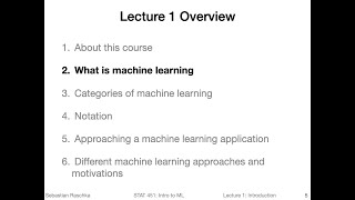
1.2 What is Machine Learning (L01: What is Machine Learning)
Sebastian Raschka
1.3 Categories of Machine Learning (L01: What is Machine Learning)
Sebastian Raschka
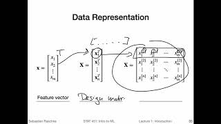
1.4 Notation (L01: What is Machine Learning)
Sebastian Raschka
1.1 Course overview (L01: What is Machine Learning)
Sebastian Raschka
1.5 ML application (L01: What is Machine Learning)
Sebastian Raschka
1.6 ML motivation (L01: What is Machine Learning)
Sebastian Raschka
2.1 Introduction to NN (L02: Nearest Neighbor Methods)
Sebastian Raschka
2.2 Nearest neighbor decision boundary (L02: Nearest Neighbor Methods)
Sebastian Raschka
2.3 K-nearest neighbors (L02: Nearest Neighbor Methods)
Sebastian Raschka
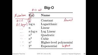
2.4 Big O of K-nearest neighbors (L02: Nearest Neighbor Methods)
Sebastian Raschka
2.5 Improving k-nearest neighbors (L02: Nearest Neighbor Methods)
Sebastian Raschka
2.6 K-nearest neighbors in Python (L02: Nearest Neighbor Methods)
Sebastian Raschka
3.1 (Optional) Python overview
Sebastian Raschka
3.2 (Optional) Python setup
Sebastian Raschka
3.3 (Optional) Running Python code
Sebastian Raschka
4.1 Intro to NumPy (L04: Scientific Computing in Python)
Sebastian Raschka
4.2 NumPy Array Construction and Indexing (L04: Scientific Computing in Python)
Sebastian Raschka
4.4 NumPy Broadcasting (L04: Scientific Computing in Python)
Sebastian Raschka
4.5 NumPy Advanced Indexing -- Memory Views and Copies (L04: Scientific Computing in Python)
Sebastian Raschka
4.3 NumPy Array Math and Universal Functions (L04: Scientific Computing in Python)
Sebastian Raschka
4.7 Reshaping NumPy Arrays (L04: Scientific Computing in Python)
Sebastian Raschka
4.6 NumPy Random Number Generators (L04: Scientific Computing in Python)
Sebastian Raschka
4.8 NumPy Comparison Operators and Masks (L04: Scientific Computing in Python)
Sebastian Raschka
4.9 NumPy Linear Algebra Basics (L04: Scientific Computing in Python)
Sebastian Raschka
4.10 Matplotlib (L04: Scientific Computing in Python)
Sebastian Raschka
5.1 Reading a Dataset from a Tabular Text File (L05: Machine Learning with Scikit-Learn)
Sebastian Raschka
5.2 Basic data handling (L05: Machine Learning with Scikit-Learn)
Sebastian Raschka
5.3 Object Oriented Programming & Python Classes (L05: Machine Learning with Scikit-Learn)
Sebastian Raschka
5.4 Intro to Scikit-learn (L05: Machine Learning with Scikit-Learn)
Sebastian Raschka
5.5 Scikit-learn Transformer API (L05: Machine Learning with Scikit-Learn)
Sebastian Raschka
5.6 Scikit-learn Pipelines (L05: Machine Learning with Scikit-Learn)
Sebastian Raschka
6.1 Intro to Decision Trees (L06: Decision Trees)
Sebastian Raschka
6.2 Recursive algorithms & Big-O (L06: Decision Trees)
Sebastian Raschka
6.3 Types of decision trees (L06: Decision Trees)
Sebastian Raschka
6.5 Gini & Entropy versus misclassification error (L06: Decision Trees)
Sebastian Raschka
6.6 Improvements & dealing with overfitting (L06: Decision Trees)
Sebastian Raschka
6.7 Code Example Implementing Decision Trees in Scikit-Learn (L06: Decision Trees)
Sebastian Raschka
7.1 Intro to ensemble methods (L07: Ensemble Methods)
Sebastian Raschka
7.2 Majority Voting (L07: Ensemble Methods)
Sebastian Raschka
7.3 Bagging (L07: Ensemble Methods)
Sebastian Raschka
7.4 Boosting and AdaBoost (L07: Ensemble Methods)
Sebastian Raschka
7.5 Gradient Boosting (L07: Ensemble Methods)
Sebastian Raschka
7.6 Random Forests (L07: Ensemble Methods)
Sebastian Raschka
7.7 Stacking (L07: Ensemble Methods)
Sebastian Raschka
8.1 Intro to overfitting and underfitting (L08: Model Evaluation Part 1)
Sebastian Raschka
8.2 Intuition behind bias and variance (L08: Model Evaluation Part 1)
Sebastian Raschka
8.3 Bias-Variance Decomposition of the Squared Error (L08: Model Evaluation Part 1)
Sebastian Raschka
8.4 Bias and Variance vs Overfitting and Underfitting (L08: Model Evaluation Part 1)
Sebastian Raschka
More on: ML Maths Basics
View skill →


Related Reads
📰
📰
📰
📰
Want to get started with deep learning
Reddit r/deeplearning
Building a Deepfake Detector From Scratch — What Nobody Tells You
Medium · Deep Learning
Unfolding the Meandering Path: High-Dimensional Invariance and the Flat 2D Plane of Neural…
Medium · Deep Learning
Implementing Neural Style Transfer from Scratch: The Project That Started It All
Medium · Deep Learning
🎓
Tutor Explanation