Intro to Deep Learning -- L09 Regularization [Stat453, SS20]
Key Takeaways
The video lecture covers regularization techniques in deep learning, including methods to avoid overfitting, with a focus on L1 and L2 regularization, dropout, and early stopping, using tools such as Python and TensorFlow.
Full Transcript
hi everyone yes since that's so much fun another recording so today I'm going to talk about regularization last lecture we talked about deep neural networks and we build our first multi-layer perceptrons and we've seen if we have a lot of parameters it can happen that we over fit when we do in the training so that basically means we train our model on the training set and then we observe that the accuracy goes up and up and up and up but at some point we see a decline in the validation performance and also the test set performance in the end will not be as great due to overfitting so that means the model may remember or memorize certain things in the training set that are not general so the the methods the or the predictions don't generalize to new data and in deploying or in general machining the whole goal is basically to make good predictions on new data so in order to prevent this overfitting there are different techniques usually they are summarized another important on regularization so one classic technique for regularization is just stopping the training early so if we observe that the validation set goes performance goes down we can just stop training it that would be one classic technique another set of classic techniques is on l2 and a1 regularization so weight penalties so in that way we add a penalty against complexity so one of these you have already heard about in other statistics courses for example l1 regularization is also known as lasso regression the other one the other popular one is l2 regression so in that way the two penalty ads quadratic penalty to the loss function this is also known as rich regression if you have heard of this and these are also two I would say not too common techniques anymore in the context of deep learning so one really popular technique that has been developed around 2013 2014 is dropout and we will talk about dropout also in this course which is maybe right now the most I would say frequently used and well used technique so let me do the screen swapping again and then let's go through the lectures one second so yeah today we'll be talking about regularization which is a technique to prevent overfitting so last time we looked a little bit what overfitting is how it looks like on different data sets so overfitting why it's a problem is because our model may just memorize certain patterns in the training set which are not generalizing to new data which will mean basically that our model will not perform very well on new data and how we can reduce overfitting is for for example by reducing the model capacity last lecture we talked a little bit about model capacity what that means you can think of it in simple terms it's just the number or the complexity of the model how complex the decision boundary can be so what types of functions the model can approximate so we can basically reduce the rate of overfitting by reducing the capacity of the model making the model simpler essentially and also by reducing this kind of tied together by reducing the variance of the predictions so if we think back of last lecture we took for example the mean square error and we decomposed it into a bias variance and noise term so by reducing the variance we can also reduce overfitting by reducing the variance that basically means that we if we if you look at different training sets we would produce similar or consistent predictions when we fit a model on different training sets from the same population if we have a high variance if there are slight changes in the data set in the training set the outputs the predictions will be vastly different on the same test data point so a variance here means how how different the predictions are if I train the model on different training sets that are still from the same population but have slight differences so how how sensitive is the model to different patterns of noise in the training set so there's a problem that we want to suppress so this overfitting is something that is not desirable so one way to reduce overfitting is by a regularization so regularization techniques also lead to the lower capacity that I just previously mentioned in the context of deep learning you can also just more general terms think of regularization as adding additional information to the training procedure so to add some some sort of constraint you can think of it as a change to the objective function for example some some additional information so and this regularization can help us with reducing overfitting by for example reducing capacity of the model so the common our regularization techniques that are often used in deep learning are early stopping that means stopping the training early before when we see a decline in the validation performance before it gets too bad we stop the training because then we avoid that over a model of it's too much a better way to address overfitting is adding a penalty to the loss function for example L one or two penalties these are the non-common norm peloton penalties which add a coefficient or a term that is depending on the size of the weights to the loss function and by that we will reduce the size of the weights which means that the model will be less sensitive to small fluctuations in a data set the third or third technique here would be drop out drop out is maybe the most popular technique in deep learning for reducing the model capacity or just preventing overfitting so we will talk about these topics one by one but before we even go to the early stopping I just wanted to give you another brief tip or how to get better performance and how to reduce overfitting that would be simply by collecting more data or or commenting the data that you already have so that is an additional point I wouldn't call this regularization but it is also a very useful technique to prevent overfitting so I would generally if you can always recommend collecting more data so the more data you have usually the better the model will perform and it is also helpful for example if you have image data to modify your data so it is not always possible so for example if you have image data for example one let me lay it on my iPad here so one possible way to augment the image data is by adding random rotation in one second things okay random rotation would be one way you can augment your data set if you have images for example you if you have if you think of the amnesty to set let's say I have my amnesty images this is a number two here I can for example rotate it slightly to the right so my numbers may be something like this now and I can also similarly rotate it to level to the left side so it's maybe like this so in that way I can from one image so I rotated here to the right and I rotated here to the left I can generate additional training data points that are very similar to my training set however these are new data points and can help with overfitting because now the model can't exactly memorize the pics of positions for example let's say we have this original image here on the Left I have a pixel use a black color here pixel in this position it may just remember okay there are two pixels here at these positions and if there are two pixels here at these positions then it's the number two however if I now slightly rotate it so this pixel may still be the same position but this one the previous pics is now here so it can't really memorize the exact position of the pixel so it has to somewhat learn a pattern or a more like an overall shape that is one way on for commenting images however you don't want to do something maybe completely crazy in turn depends of course on your application but you maybe don't want to completely rotate your image that may not always make sense so there are certain I mean ways where this may make sense for example if you build an ATM machine and you want a machine to read the number whether the check is upside down or not that may makes maybe sense but it wouldn't make sense Ritu mirror images in that sense via numbers for example if you think some space left here if you have the number two here you don't want to you don't want to heart drawn mirror too you don't want to flip it basically because this is something you wouldn't encounter in real life so this is not like a real number so that way you have to be also a little bit careful about what types of modifications you consider for example for face images it may not make a huge difference whether you flip the face or not that makes maybe sense because it depends how your camera works some cameras flip produce mirror images some don't so in that way maybe that is something that's okay but you don't want to create like these weird numbers by flipping numbers otherwise how you can generate artificial data points is for example by cropping so yeah cropping that means simply that we if we have another number here say this is our original amnesty image but I can do is I can resize my image I can make it a little bit larger for example like this and then I can crop out a random region from this image it has the same size as the purple region so let's assume it's the same size I can crop a random region and this is basically our equivalent to just translating the number of pixels to a different position so this has the same effect as if I would have put the number two here so what there's a resizing and cropping trick is computationally a little bit cheaper than computers so just moving the pixels over so that is one way you can do this but you can also of course crop it in a way that you get a smaller image smaller random image so that would be another way you can augment your data set of course this doesn't really make sense with other types of data sets if you have text it's not much you can crop on one or certain they also certain certain things you can do with text example maybe introducing some typos maybe changing single letter in a text or something like this with a certain probability or also just the capitalization of letters you can maybe randomly capitalize the letter or not but that also again depends on whether your model uses uppercase lowercase information and this is always something you have to think about in a case-by-case basis for some datasets it makes sense and for some datasets it doesn't make sense but let's go back maybe to the first term collecting more data is always a good idea so I mean it does not always help a lot but usually it also can't hurt here so if if you can it's usually always recommended and one way to find out whether it really benefits you is by uploading a so-called learning curve so this is called learning curve what a learning curve is is basically a plot as that plots the accuracy for different training set sizes so here what I was doing I was taking the M this data set but only a subset because just to on because it took a little bit longer to compute on my computer and just to show you an example so this is a very small subset of M list what I did here is I have a constant size test that so I keep the test that size constant I have to admit I forgot the number but I think it was on for 5k it doesn't really matter I'm just showing you constant test set and then what I'm doing is I'm increasing the training set size so I start with a very small training set size could be I think I was like what I said here was 100 and then I'm creasing it up to 3,500 and I can see here when I increase my data set size so my training performance goes down so this is you've already seen the softmax model this is the softmax regression if you remember there's like multinomial logistic regression its logistic regression with for multiple classes so if you remember how it looked like it was something like this everything was connected to everything so it's a linear model a generalized linear model this is the inputs are the number of pixels in the image if we have M nest is 28 times 28 should beam sir 84 input pixels and a number of classes here this is so say C is the number of classes it's 10 because we have the digits 0 to 9 so we have 10 different digits it is a little bit weird that the training performance goes down I mean is this is generalized linear model usually training performance would also go up it doesn't really matter here can for this plot the training accuracy really doesn't matter it's just something you can ignore however what you can see here that's the most important part in this figure is that the test set performance goes up that means if I would collect more data for example if I would collect 4,000 or 5,000 data points what I would expect is that this would maybe not so steep but it would still go up it's in a way it tells me this will on help me collecting more edom would help me getting a better accuracy if I collect more data usually also this prevents overfitting so I'm not sure I think this is because just a generalized linear model but the Dex cats and dogs example I showed you last time it would be more something like where we have a training set that starts here and then usually over time the performance gets better also but then also you get this increased overfitting rate but even though the overfitting is bigger here let's say then here you also want to care about the overall performance for example of this threshold here you can see even though in this part I'm fitting more than here still get a better performance compared to before here so in that way it's usually a sweet spot between on improving the overall performance versus reducing overfitting but we will see another example of that later with the cats and dogs example okay so here are some examples for augmenting images so at the top this is the original m-miss data set so you can see I mean this is just 28 times 28 so it's a little bit pixelated but 7784 it's worried a big data set still so if you think about images that we work with if you take a camera picture it's what the resolutions are these days but let's say 1,000 times 1,000 you have already 1 million pixels so it's a huge data set so it's easy to overfit in this lecture we are just working with multi-layer perceptrons just to keep things simple in after Spring Break actually we will talk about convolutional neural networks which are models that can deal with such data much much much better in any case just to focus on data commentation for now so I'm showing you an example here of the MLS data set just for random numbers or data points so here I have a randomly augmented version of these images and I should mention the augmentation is random so every time I run this it will do something that is slightly different within a certain range for example I can say rotate my image in a range between let's say minus 20 and 20 degrees so it is always a number between those two it's not always the same number this is kind of useful because that allows us to almost create infinitely many versions of that image also one more thing I wanted to say here is I have two versions of this so this this randomly augmented version and this recommended version here the only the big difference is that in the middle row I'm just using oh sorry at the bottom row I'm just using the default settings and you can see this two and this one they are even this is very extremely in the nine you can see it's more accelerated than this one it may be a good or a bad thing but I think this is maybe a little bit too extreme this is just how punctual how how this rotation method works so if you want to get a little bit better quality there is in the Python imaging library this bilinear filter that you can or interpolation method sorry it's a temporary method this will help you to get a little bit better results in the center row I was actually using this PIL image bilinear thing to get a little bit of a better performance if you want to get the code examples for that it's all on github and I want to really go there because it's kind of boring I didn't want to just execute the code because it's there's not much to see so I just made a screenshot of the relevant part which is the transformation so in PI torch this is torch or poach vision is kind of part of pi touch it's a separate Python library but if you went to the Python dot orc website maybe let's just do this easier to show so when you yeah if you already installed Python which I think you already have because you needed a torii for homework I recommended you to select the installation command based on your computer of course and let's say you selected let's say you have a Mac computer and you selected the Condor one python version with CUDA 10.1 or it could also be just no GPU it will give you a command here that Orion if you have seen that it will already include torch version so chances are you have it already installed so you don't have to worry about installing it separately since we are already in a browser we can actually go to look it up here and then class repository and we are talking about regularization this coach date augmentation so this is not very exciting code here so all I'm doing is I'm importing the taught revision packages so I'm actually importing two things towards vision and torch vision datasets so in the data sets up library they have some datasets available like Amnesty so you don't have to download it manually so it's providing you some functions to load that more conveniently that's mostly for benchmarking however in the project you will likely work with your own data set and for that you need to use your own data loader methods but homework 3 explains you or shows you an example of how to load an own data set that is not part of this data sets library but I'm getting distracted here again so let me talk about touch vision and not the data sets for now so what I'm showing you here is to transform methods so I'm building my own transformation pipelines using torch vision because taught you shion's taught revision dot transforms don't compose and the compose method lets me compose number of rotations or sorry a number of transformations whatever I like and they have a lot of options there in this library I'm just showing you some of them but if you go go to this website they have a whole range of things let me see probably add it a lot more recently so there are a lot of different methods may be helpful to just scroll through this and see what all what kinds of things they have here but the major ones I would say is a random rotation resizing and random cropping there's one method random affine that does multiple things in one so this is the one that I've shown you in this slide and always so these are methods that are executed on PIL Python imaging library image format so here the data is still in an image format however for pi touch we need to get that into a tensor the potage tensor so this is what this method is doing it will convert the image into a tensor one side effect that I sometimes forget in the beginning when 2017 when I was using other tools and then PI touch was new and I was sometimes over normalizing things because one thing to keep in mind about this it's already scaling the data into a zero one range I don't know why they do that maybe it's just um I don't anyway so it is an automatically normalizing mimics scaling the data into the zero one range if you if you execute this two tensor command for image data it's always in general it's helpful to have data centered at zero so that you have positive small positive and small negative values that's because you also have the weight usually centered at zero and it just we will talk more about this will help optimization so here what I'm doing is I'm also normalizing my images such that they are centered at zero and will be in the minus one one range so let me go actually back to the slides because then I can okay so going back oops so going back to the slide here I'm just to again show you what's going on here so this is just the screenshot of what I've shown you just in browser so at the top I have my training transformation and at the at the bottom this is what I'm using for the test set so for the training um we have this random of fine but this is just really a convenience function wrapping all these three together and here's some randomness so we have these random modifications whereas in the test set we have deterministic behavior but again back to the nominalization here this is the z-score so one more thing is this is just called normalized but it is called Z so ah normalization which is basically what we know as standardization from the previous machine learning class and organization and what it is doing is it's basically rescaling our data such that it has zero mean and unit variance so this is usually helpful because then our data will be centered at zero can have small positive and small negative values similar to how we initialize weights weights are also initially initialized such that they have small positive and negative values and this usually helps optimization algorithms and we will talk more about optimization algorithms in the next lectures here what we are doing is we are rescanning it with these properties such that if we use so maybe I should write down the operation so X prime assume is the modified or rescaled training data point and we rescale the given data point this is actually also for a given feature so let's say this is for pixel by pixel shouldn't have this we subtract the mean first and the mean is computed as the average over all images in the training set for this pixel location for pixel I and then we do the same thing for the standard deviation again the standard deviation is computed over the whole training set and this is for the eyes pixel so this is how we standardize a given pixel and if we do that after the standardization the pixel position have will be across all training points be centered at 0 with unit variance and Y so in this case actually what will happen is that the range will be minus 1 to 1 so normally if you have a data set you have the spread the cinetic vision so it can be usually values larger than minus 1 or values sorry sorry smaller more negative than minus 1 or larger than 1 here it is bounded by minus 1 and 1 though because we already normalized images using this normalized function here so why is that why is it minus one to one I mean it's just easy to see let us plug in some numbers here so if I consider this equation here or this formula here and then I plug in for the mean the minus 0.5 I'm taking it from here so I'm plugging this in here and then my denominator I also put the point 5 we're just coming from here and then for the pixel I put in I mean the pixel numbers could be between 0 & 1 so let's put in a 0 here first and 0 minus 0.5 is minus 0.5 divided by 0.5 this would be minus 1 and if I have you right on the left corner here if I have pixel value 1 I subtract 0.5 then I divide by 0.5 this would be 0.5 divided by 0.5 which is 1 so in this this is why the boundary for the values is between 0 minus 1 and 1 in this special case just this is just a side effect of this normalized function also I should mention in practice in practice these values are derived from the training set so in practice we would compute the mean and the standard deviation from a training set this is like I would say most correct way to do this but it doesn't honestly doesn't really matter in terms of the network performance if you choose constants it's usually fine if you are look at beta we will do that at transfer learning methods for pre-trained models available at st. watch vision you will find for image net they estimate numbers like four point four something so it's usually pretty close to 0.5 but or of course it depends on the data set but it doesn't really matter here and also here just for simplicity we use point five let me clear the screen a little bit because too much drawing here this one more thing I want to say and this thing I want to say is that we put one value here and one value here for the mean and the standard deviation and this is because M this is a black and white data set or grayscale data set so if we have the dimensions of also and it must write it like this so this is oops a matrix of real values each image is 20 by 28 times 28 matrix but we also have a color channel so it's usually a 3d tensor so 1 by x 28 times 28 tensor so the one here stands for the color channel so you only we only have one color channel here which is why we only have one mean and one standard deviation so we use so we compute them usually separately for each channel and here what we are doing is we are putting in a couple however if we would have a data set that has multiple color channels or multiple let me see so if we have a data set with multiple color channels for example R GB we would have three for example in this case this would be three colour channels so we would also have three mean values and three deviation arrows if we standardized by color channel which is what's very common for images if you have a tabular data set you would actually normalize this by a feature value by each column in the data set so here we are normalizing by each color channel so we can have a different mean and different station okay so one more thing I'm seeing this year at the bottom this is actually very important so you've already seen that we have data Laura's in Python and for the data loader we provide a data set and the data set is just a class the data set class that defines how a data point or image can be opened in Python here we use something else already Intuit revision this data set sub package where there's already missed data set contained and all we have to do then but for the data Laura so is to provide the training data set and for the training data set or for the data set in general we have an optional transform method or a chain of transformation commands and these are our commands that perform this data augmentation so these are the different ones that we define and we just provide these transformations to the transform argument here and then it will apply all these transformations for us so now this is for the training set if I have a validation or a test set for example let's assume this is the test set I will also just change this to test transforms which are this here basically so that's all we need to handle training and test sets separately and it looks maybe little bit confusing I was doing a lot of drawing here but it's super simple in practice as you see in homework 3 it's actually not a big deal it's pretty easy to do go to the next slide and if there are no questions but haha you can't ask questions no you can ask questions in on Piazza and we'll have office also you can ask more questions because this is like a little bit unfortunate that we don't have this interactivity here so we have to rely on other methods for asking questions I will also maybe make some smaller quizzes to see if you if everything was clear or maybe what what parts need more explanations okay next slide okay see here I'm just again letting you know for RGB images you want to put three numbers in here because you know have three color channels so we talked what time is it may we talk like us an hour what data augmentation but the real lecture is about regularization so so you're reducing the network capacity and early stopping it's the simplest part about the simplest method of regularization so we are entering now the part two here where we talk about reducing the network capacity so one way to reduce the network capacity is simply to choose a smaller architecture so making the network smaller using smaller hidden layers using fewer neurons and also adding few hidden layers so the simpler the architecture the fewer parameters you have and the fewer or the lower the chance that you will over fit another way so this will will be one way to an to decrease the capacity of the network the other one is to enforce smaller weights the two penalty for example is one common method you probably heard about this in the context of other subjects such as six classes as a method called rich regression which adds a penalty to the objective function and this makes the weight smaller basically we will see how this works in detail another way to reduce the capacity and enforce smaller weights is early stopping so it's a little bit unintuitive why does it enforce smaller weights I mean it's just more like an intuition that it can enforce smaller weights because if you train your network your weights get updated all the time so they go in either direction and if you train it over fewer epochs there are few updates and you can maybe hypothesize the few updates you have the smaller the magnitude of the weights so because you don't push it into these extreme regions but of course it also depends on the learning rate and many and many other things and also it does not mean that you have a small always a small wait what it does though if you have its droid like this if you have your let's say accuracy here and this is your number of epochs so if you have a valid and so let's draw the training set performance let's say and goes like this this is one training and then for the test set performance or validation set performance you will see it will start maybe here and then you will see it goes maybe not quite as high and then at some point it may even go down so this is for the validation so we maybe want to stop at some point I mean this is something where you have to run the network to really see how the method performs but then maybe this would be a good stopping point here if this epoch you would stop the training so you would run the whole network but imagine you just saved checkpoints of your model you would reload this model and then you can evaluate it on the test set I've done it so you hypothesize here's a small overfitting it's overall good performance and this is your hypothesis maybe the best model in this range here okay that would be one method for reducing the capacity and the last one maybe the most popular one is the dropout method so to again start or go back to the early stopping principle I think I actually wanted to explain this with a few slides I was going a little bit ahead and was drawing something but again let's go through this slowly so what you do is and I would always recommend that you take your data set and divide it into three parts so you have a training set a validation set and the test set how big should these parts be I mean this kind of a little bit arbitrary depends also on the overall size of your data set but usually it's I would say good recommendation to use something like 80% for training or maybe I would say 15% for testing and 5% for validation validation it's maybe the least important part I mean all of them of course important but the more data you have for training as you've seen earlier when I showed the amidst softmax plot the more data you have for training usually the better for the model and you also don't want to have a very small test set because you want to have a test that is an unbiased estimate of the generalization performance but of course it can also have a high variance so loud you want to you can have fluctuations basically depending on what data point ends up in the training set and in the test set and a larger test set will shall essentially give you a more reliable estimate of the generalization performance so you want to have a relatively large test set so also people believe your results when you let's say write a paper but you don't want to waste too many because then your training set will be too small and then the model will not be good so it's in practice a trade-off you want to have as much data as possible for trainings for training but also you want to have a relatively large test set so your estimate of the performance will be somewhat reliable yeah so you divide your data set into three parts and the training set is for the model fitting so you fit the weights and bias units based on this training set here and the validation set is something you use during training to estimate the performance already during training but of course you will experiment with different hyper parameter settings you will change the learning rate you will change maybe the architecture you will change the number of epochs activation functions and what-have-you so if you use the radiation said every time to ever write the model you kind of leak information into this procedure so in that way because you reuse the validation set it will not be an unbiased estimate of your test set anymore this is kind of somewhat related to hypothesis testing when you do a hypothesis test multiple times until you I'd say find a p-value that is smaller than your desired significance threshold at some point if you test on the same data set multiple so if you conduct multiple tests at each test I mean how tests work for example is you have probability of observing the data given given the null hypothesis so that there's no effect if you repeatedly so with this usually you set a significance level of 0.05 so you have a 5% chance that you observe a value that is extreme as the observed one the data or more extreme 5% of the time have a type 1 error of 5% but you inflate the error if you do multiple tests basically also the more tests you do so you can think of it like this if you have this five percent error rate the chance that you don't make an error is 0.95 and now assume you test something seven times we do seven hypothesis test so the the chance that you don't make type one error is this number I can't compute this in my head here right no but it could be point seven so um yeah and then the chance that you make at least one error that you are wrong at least one out of the seven times is then simply one minus this value I know what what number this is kind to the math right now in my head but let's assume this is some number between I don't could be 2030 let's just go with 25 well check after this lecture was probably the super off but there's it say a certain a certain don't take take this with a grain of salt and but there's a certain chance a higher chance that you make a mistake if you do something multiple times and then some what I mean what we are doing here is not a hypothesis test its but it's basically the same the same issue that if we test multiple times we increase the chance that we just select something due to chance so the validation said it's not super reliable in terms of the true performance of the model the generalization performance on all possible data but it is a pretty good guess so this guess is actually better than the training set of performance guess goes from the training set we can't really tell whether something is memorizing and the model is memorizing data or not the validation set it's not used for training nor for fitting these weights and vices so it's somewhat more unbiased but it's not totally unbiased because we use it for model selection we use it for hyper parameter tuning and we use it multiple times which is why it's always important to have separate test set all right okay so here I have a plot again so this is actually what I've drawn before so this is a plot shows you the accuracy for different epochs and so increasing number of epochs and you will see usually that the training set performance will go up over time and the validation set performance will usually go down there will usually be a point at that point you will see that you get the maximum validations of performance but then you will see the performance will go down and usually this point where before it goes down is a good point to stop and again so here the overfitting is less then here however we are maybe still more interested in this point because it has the highest overall performance in terms of the validation set performance I'm not showing you a test performance here but my guess would be a test set performance it would be usually a little bit lower than the validation set performs because like I said the validation set is a little bit biased because we are select our models based on the validation set so sometimes it's just like we are lucky that we get a good performance on the validation set and we select the model specifically on the trainings test sorry validation set so on the test set it may not achieve that good performance as on the validation set okay that is early stopping and maybe the simplest technique for fitting however I mean this is not a bad idea but we will look now at different methods that help us to kind of shrink this overfitting on range so I go back and write a little bit okay so the methods we are going to use they will try to shrink this region that is the overfitting here what will happen so our goal is to 1/2 a validation set performance that this may be somewhat like this closer than training say but of course it will not always be perfect but we will aim to reduce that one danger with that though is if we reduce this overfitting too much if we are too strong with our regularization what will happen is that we will decrease both the training set in validation set performance so what we Macy's drinks at performances no something like that and the validation set point says maybe it's not overfitting that much as you can see but it is overall so you know overall it's lower than before so we don't want to add a very very strong regularization because then both the training set and validation set performance will not be as good anymore however we want to also still reduce this gap so we just hope the debilitation set performance without overfitting is now better than with overfitting so one way to achieve this is with adding norm penalties to the loss so there's l1 and l2 regularization so how that works you probably have heard about this from other statistics constant so there is a Laster regression and this is the l1 penalty and there is rich regression which is the l2 penalty so these are both methods that we sometimes also call weight shrinkage or penalty against complexity that simply means that we keep the weights small and with small weights the decision boundary will be simpler because then there are less so input data points have less influence on the decision boundary because remember when we compute the net input so we usually have an activation which is activation function which takes in some value let's call this value Z and Z itself is computed by the weighted sum of the inputs so we have usually the weights it's same in a generalized linear model or in general we have let's write this properly so we have our training set and then our weight matrix so here we have a weighted sum let's also add the bias vector so weighted sum and if we keep the weights small the decision boundary will be less susceptible to small changes in in X for instance so in that way we have a simpler decision boundary if we have smaller weight values especially if some weight values are close to zero or even zero then these weight values don't play a role at all and that will again lead to a smaller or simpler model model in a smaller model complexity because fewer weights play a role in determining the prediction okay so how this works is that we simply add term to the loss function this is the term for a two regularization which us to reduce the size of the weights and at the top I'm showing you the cost or loss function in general so sometimes I use this terminology that call the loss on a single data point l or loss and if I speak or talk about all training points all n data points I call it the cost the cost is basically the averaged loss overall data points over the whole training set y hat is as usual my prediction and why is my true class level and this is depends on what model we use could be the mean square error that we had this could be the MSE or it could be the negative log likelihood doesn't really matter so the same concept applies to both the mean square error or negative log likelihood or cross-entropy it's the same thing so it could be in some arbitrary loss function and what we do now is we add this two term and the i2 term is simply so here let's imagine a generalized linear model like logistic regression so these are my inputs and then I have something like that that gives me my hand so these are my X's and there are some weights and this it's drawn shown by this unit this is my linear model so I have these weights the weight vector so the weight vector contains here J weights so let's go W 1 W 2 W 3 up to W J and so sorry this is let's go let's say we have M weights and this is if I pick one of them it's a J's weight so we have M weights so what we simply do is we square and sum up the weights so this is writing this is equivalent to W transpose W just squaring all up these terms and then having this lambda coefficient so this lambda coefficient is just arbitrary hyper parameter so what wrote this actually here this is a hyperbola that determines the strength of the regularization of course the larger this lambda parameter yes the larger this this term becomes so large lambda means like a large penalty term and I'm also averaging over the number of training points because I'm also doing this in the loss function you don't have to do that so you can she cancel this one in this one so the mean square error will become the sum squared error but usually I like adding these averaging terms here because it makes a training more stable for example if you change the mini batch size you don't have to recalibrate the learning rate that much because so because what we do is when we compute the gradient updates we have an update that is W plus the negative gradient times we can also subtract the gradient times the learning rate so the lost gradient with respect to one weight so if we do that then we usually choose the learning rate that's called a flowing rate a term or sometimes we also say alpha doesn't really matter so for this learning rate here we have to choose this carefully to converge and since this is a multiplicative factor it is so we have this one-half here this one-half will also appear in my derivative and my loss the rotor so if I have what it basically means is you have more data points here because of the sum the law school or the cost will be larger when I have more a larger mini-batch science and if I have a larger cost then I have to reduce the learning rate so every time I change my mini batch size I would have to fine-tune my learning rate again of course you always should find you in the learning rate if you make changes however it's simpler it's more stable if you have this averaging term then it's less susceptible to changes in the mini batch size what I wanted to say here is yes so we have this squared term here I think I may have not even mentioned that so that means this whole term will become bigger this whole term that we add to the last function here this whole term will become bigger as the weights become bigger because this is sum over the squared weights so it will become quadratically bigger with the larger weights let me clearing in the slides because it's getting messy in here so so the bigger the weights the bigger this term becomes and if this term becomes bigger the weights become bigger then also the whole cost let's just call it loss becomes bigger and again remember our goal is to minimize the loss so in order to minimize the loss we have to minimize two terms now we have to minimize the prediction performance so how close we are to the true label but then also we want to minimize the second term which is the size of the weights so ideally we want to have this zero because then this won't affect the loss but if we have a zero weight I mean it will be likely that this will be a very bad prediction because Y hat depends on the prediction where this is again w team explains bias so if we have zero weight we'll have a very small penalty for the size of weights actually actually zero but then again our predictions will probably not be good so there should be a sweet spot we want to minimize the prediction error but also at the same time we want to minimize the weights so we want to minimize two things now so that is l2 regularization l1 regularization is pretty similar the only difference is that instead of using a square charm here so we squared size all the way we use the absolute value here and we won't go into too much details here of what it does exactly so there are lots of books and papers written about that about lasso regression so here or in general the key ideas that it encourages sparsity and sparsity means that many values in the weight vector can become zero so the stronger the leg of organization the higher the chance that you will have higher the number of 0 weights so in the so a two regularization just shrinks the weights and this will in addition force the weights to be zero so you you can think of it it can be useful for feature selection even so you select features using lasso regression but you cannot choose which weights become zero so it's also kind of limited if you have so you can't choose the number and which weights become zero so in that way it's not really the same as feature selection but it is it can be useful to reduce the complexity of your data set so if you've a weight vector the weight has say w1 w2 say we have own for weights in this weight vector there's a high chance with last regularization that that said two of them becomes zero and if it's just convention and computer science we say or in general say if linea drive more than half of the elements in a vector or matrix are zeros then this is a sparse matrix or sparse vector but of course this is just a con loose convention what sparsity essentially means is that there are many zeros and a one regularization yeah encourages many zeros the one advantage of course is disadvantages of course this is not differentiable so with the l2 regularization so again when we do our grain in the send we want to compute the gradient which we use then to update the weights if we have now a modified cost function or loss function but we also have two different so let me go back here maybe in a second okay so what I wanted to say is so what we usually do is we compute partial derivative of the loss with respect to the way to update the weights with gradient descent before we were just computing the derivative of the loss function for example the derivative of the mean squared error now we have to add this penalty term we have also to derive that and if you probably know it's the simplest for simplest rule in calculus the sum rule so if we have a function and it's not same composition of two another composition a sum of two functions let's call one giving GX so if we want to derive this one we just derive them separately that's some rule so in that way what I'm trying to say is we can just derive this term separately and add it to the derivative of whatever this is depends on the last function in order to compute the derivative for this part I mean it's pretty simple we use the power rule we just bring this one forward so it's true lambda over m and then some what about you that's basically it write something look so this would be basically our simple penalty term that we end and this is nicely the roof differentiable because it's just square that's not so nice here because we have known absolute value no of course we can use tricks like the one that we use for the reloj function but I would just say this is usually a little bit harder to optimize because like a smooth function I get read function and so with a creditor crunch again we have let's say some value mmm it's call this P for penalty or something like this size of the weights so what we'll have in a two regularization of something like this and al1 regularization we will have something like this so it won't be that smooth and yeah talking about this I think I added some slides to explain you more behind the intuition yeah I did so yeah there's some quick geometric interpretation of a to regularization so here what I'm drawing is a surface plot so there are two XE - you have two x is w 1 and sorry WI and W J and these are both two arbitrary weights just assume I have a linear model journalist linear one on the logistic regression or let's say even add a line with linear activation function so this is I have multiple weights so each connection is a weight and I'm just picking two two of them so let's say I pick this one and this one so I have my W I am i WJ here and in the surface plot this is the contours represent the loss so this point in the center this is the minimum loss so this is where the losses is the minimum value that's the point that we want to get when we optimize the last term when we optimize say 1 over n let's just not do the 1 over n just for one date or maybe it's better ok so if we want to minimize this term the loss or cost then if if this is minimized we are here in the center point of the surface but in the further we go outside the larger this value becomes so before this was our regular optimization objective now in addition to that we have this penalty term which is what was lambda and then sum or squared weights so we have this additional term and this becomes larger the larger the weights become so I'm showing you the second term via this second control graph and the penalty or loss will be exactly zero for that weight if so this is the gray shaded area is the loss for the second term and will be zero if the weights are zero because then we have a sum over 0 which is 0 basically so in that way I'm so that would be if we add 0 so that would be the optimal for the weight penalty that would be optimal value and we minimize the second term however if we minimize the second term we have zero value here but we are very very far away usually from the minimum loss value this part and again if I go back to slides so we want to minimize this thing and this thing so and there's a sweet spot so if I only minimize this thing then usually this other thing will be large so we have to find a sweet spot and it turns out for a two regularization this sweet spot is of course makes sense it's usually somewhere in between and it will be usually a weight that is smaller then the weight that we would get without the penalty so so you can see this is more to the left so it's right here so here we have a relatively large weights and if we are in this sweet spot the weights are a little bit smaller so the axis again are representing the sizes of the weights and it's just the geometric interpretation of this so we want to find a good sweet spot between having small weights but also minimizing the loss function this is for l2 regularization for l1 regularization this looks relatively similar but now we have this diamond-shaped thing the same concept applies we want to find a sweet spot between minimizing the loss and minimizing the size of the weights however it turns out that often the compromise will lie on one of these axes so it will lie either here or here and if that happens one weight will be here in this case zero so that is the main difference between the two so this one will encourage like these zero weights what's next okay so I was talking about generalized linear models logistic regression and so forth of course though we work with multi-layer networks so what we have is the difference is basically here we have a matrix now it's a weight matrix so before we had a weight vector so matrix consisting of let me draw it like this we usually have M columns where m is the number of features in the previous layer and then we have Oh shall I call this let's call this H the number of values in the next layer so then usually what we do is we have oh this is our data training data set so this is usually n times M and then we multiply it by W transpose and then this is our weighted inputs and so forth so we have this weight matrix now so the multiple weights and in how we use weight matrix for regularization is pretty simple we just use the Frobenius known which is just summing the weights over the columns and the rows and we do this actually for each layer that's all we need okay so here I have also what I already drawn that before the update for grain descent so here it's for one data point so the only difference I have here is that we this is for one particular weight sorry so if I have it shown for one weight I and J so this is one so if I have my weight matrix this is one weight in the weight right X so if I update this again regularly I subtract the loss with respect to that weight times the learning rate Etta and now when I perform my update with two regularization I add this penalty term and actually the derivative of this penalty term this is a pretty simple it's like I said before so if a penalty was I J squared and then lambda 2 and so it's correct mm-hmm so just for for one weight so we just simply update this by using the power rule so we bring the two here and this is all we have to do it's a quadratic term it's pretty simple to derive and then we just add this to our loss function and we apply the learning rate to both of them and this is all we need so how does it look like in tight works so here I'm going to show you three ways now to do regularization pad watch so there's l2 regularization for logistic regression doing it manually then doing automatically and then I think I have a short one where I do this for neural networks so let's go through it one by one okay so in this first one let me let me open this okay this is the code notebook I just clicked on the link and the slides and this is a very simple notebook I prepared to compare a logistic regression with two regularization doing it manually and doing it automatically I did it both ways so you can see that both reproduce the same results for instance here I have the weight paratus after regularization which are one point seven five four six and one point five nine nine seven and if you go down a little bit the automatic so this was the automatic way sorry it gives you these parameters and the manual way they give you the same parameters so just to double-check that my manual approach is actually doing what is it supposed to be doing okay let's not scroll around too much here and go through it step by step so in this notebook I'm simply loading a very basic simple super simple data set it doesn't really matter because I just want to get some results to see that regularization is implemented correctly so this is a very simple logistic regression model for binary classification I just have one layer because logistic regression we don't have hidden layers it's just a layer connecting the features to the output there's only one output in a logistic regression again this is just to zero the weights and biases it's not really necessary but since it's a convex cost function we don't really need to start with random weights and then we also only have our single sigmoid activation that is all what something that have seen before it's nothing new the new part here is in the training so what I'm doing here so I'm showing you the automatic way so what i'm doing here is implementing logistic regression regression with regularization and like I mentioned before a to regularization is much more popular in deep learning compared to l1 regularization so there is dedicated parameter of the optimizer there is the STD the so Casa Grande is an optimizer that we used before and it has a weight decay parameter and the weight decay parent is actually implementing l2 regularization and here we simply provide the lambda term the regularization strength and what value this should have I mean this is hard to say it depends on the data set the pain depends on the model and the model capacity and usually this is something you have to find out why up high performance or tuning maybe you want to start with 0.5 and then see whether making a larger or smaller has the beneficial impact on the overfitting rate so reducing overfitting by addressing or changing lambda but then also you want to see that the validation accuracy doesn't go much doesn't become too bad either so like I said before there's usually also sweet spot finding a spot where you have moderate regularization that the training accuracy and validation accuracy remain high but that you also reduce the overfitting and that is all we need to do so I have my binary cross-entropy here and that's it there's no further change required let me maybe go through the slides though because there I can draw here it's a little bit hard to explain things just by highlighting it let me go back to the slides so the slides I was just simply copying sections from the notebook so the MS so that I was just showing oops I'm sorry that's always when you do things life okay so I was showing you things for the automatic approach where we have this weight decay parameter in our argument function argument in the SGD optimizer and with that it will we perform the regularization for us which is exactly equivalent to doing it manually this way this is what I had in the notebook as well section so the lower section of how to do this in in the manual way what I'm doing again is I'm computing the cross entropy the binary cross entropy for logistic regression again remember this is the negative log likelihood and here I'm just computing the the penalty term when you remember the penalty term was for regularization was this lambda over N and then W I J for the J's weight and this is the penalty term so here though one thing I should say is I'm using the sum of the losses functions so I'm not using the average so here I specifically said some so in that way there's no averaging going on so all there is it's just the summation of all the weight terms which is being done here so this is w transpose W so what we will do is we'll just compute the weighted sum of all the weights so if I have a weight vector that consists of it's a w1 w2 w3 what it will do is simply compute W 1 squared plus W 2 squared plus W 3 squared so I'm just computing with a stop product here I'm computing the weighted basic the credit ik Trump's summed up multiply it by my regularization strength lambda which is maybe a value between 0.5 I have to check it might not book what I actually chose there but doesn't really matter another thing I have here is the 0.5 coefficient where does that one come from if we go back you go big here okay so when we go back here this is my regularization term and like I said we use when we compute a derivative we just use the power rule we bring the two up front here so it's actually two times lambda over N sum J W J okay so here the two sorry the two will go away so the thing is it may be a little bit annoying to have this two so you have two times lambda or it can be confusing so in that way usually we add a point five in front of it so instead of writing it like this some computational tools assume you have written it as this and then the squared so what will happen then is if you use the power rule you put the 2 here then it will cancel each other so you have this one and this one cancels so that is actually what's going on in pie chart so pi table does this by default and this if I go back this is basically the 1 over N 1 over 2 sorry which is the 0.5 that we are seeing that we are seeing right here this is so like I said I wanted to reproduce the results that packaged up or give us automatically so I have to do this if I want to get this exact same results as with the automatic approach but it's not really necessary another aspect is that pie chart is normal or regular rising the bias unit as well so in order to reproduce the results you also have to consider this bias term in patrasche the biases just treat it like a regular weight this is I mean this is fine if you use deep neural networks it's a little bit weird for generalized linear models it's not really ideal so if you want to implement logistic regression with paid watch I recommend maybe not using the automatic way doing the manual way and then also getting rid of this term if you use Python implement linear regression regularized linear regression for example rich regression the reason why we don't want this is if the bias is regular rest you lose the intercept and I mean this is fine if you standardize your data with mean zero but if you have not then this can be a problem for example think of think of a regular linear regression for now so let's say I have my target variable in linear regression and some dependent variable my predictor variable or my future variable X and then let's say between the target and the features the data points look like like that so as you know the bias unit is the intercept the y-axis intercept so if I have a linear regression model I may fit the data like this just the hedging this would be a super straight line but now let's assume I regularize the bias what will happen is that the bias will be also becoming smaller forced to towards zero so what will happen then is if my bias goes to 0 so if I move it this way what happened this is something like like this should be a straight line sorry it will look like like this maybe because it has it kind of forces the bias to be zero or close to zero and then I can really fit this data in well anymore so that way this is why we want don't want to regularize the bias we don't want to really change the intercept but again if you standardize your data so if you have exactly the same beta and you used to z-score snide as a normalization which was like this X prime X minus the mean divided by the standard deviation if I do this to the data set on the Left what will happen is they will be different it will be centered at zero somewhere and then I don't need this intercept term so in that way I don't care whether the bias is regular right or not because it will be zero anyway but in general I think it's most of the time a good idea not to regularize the bias in pi touch they do this it doesn't matter for the deep neural networks but for simpler models like linear regression or lasso regression or rich regression it would matter okay so this is if you do it manually this is just implementing the equations that we have talked through and if I do this in pie charts again I use this weight decay apart up and set it to lambda okay oh yeah so this is a question for you why is the bias usually not regularized which I think I just explained to you so that is a pretty easy question but yeah it still doesn't hurt to ask yourself the same question before the final exam maybe it is the question in the final exam who knows so now I'm showing you regularization for neural network that has more than also that has one or more hidden layers that is where we use the Frobenius norm this is again super simple to implement this very similar to before except that we have a weight matrix so what I'm actually doing instead of going on with the rows and columns I'm applying this regularization to all model parameters which is the weights and the biases like PI toward us just summing them up and one more thing is what I'm also doing here is I divide by n so the targets dot size zero is n number of data points in my mini batch or training set depends on what the features is if this is a mini batch it's actually it is a mini batch and the mini bench sighs so this is then exactly like the equations we had on the previous slides and this is required now because I'm not setting reduction to sum so I'm not setting it to some and by default if this is not set to sum it's the average so this is why I'm also applying this M here anything else interesting here no I mean this is exactly the same as before except now that we have weight matrix instead of a weight vector I just iterate over all the parameters because it's just simpler to express in code okay oh I just answer this question already for you so the target set size is just the 1 over N and like I said before in neural networks it doesn't really matter whether we recognize the bias or not but if you really don't want to regularize the bias then you can also do it like this it's a small modification so here I'm stead of before I was just iterating over all parameters now I'm iterating through something like a name parameter list so we dictionary so here I access the practice by name and so this is a couple of dictionary where you have a name and then the parameter value itself P is still the parameter value the name is now named like bias or weight and I'm just checking whether the name contains the word weight so whether it's a weight or not and if it is a weight then I apply my regularization again so this is exactly the same as before except that I'm not specifically only choosing the weights and not the biases just quickly here so yeah how it would look like I mean this is really exaggerated so just assume you have a model with a very strong in a very weak and the moderate regularization strength and this is really exaggerated so it won't look that extreme but assume you have a data set like here in the center and you have low regularization on no regularization so in this what will happen is that your decision boundary will be relatively complicated so what it means is this is very complicated in shape so this is fitting the data very closely I'm writing high variance here because if I would have a slightly different training set so if I would have for example the training set let's say just maybe shifted a little bit like this the decision boundary would look different it would look maybe like this so in that way it's very susceptible to how the training set looks like if I would sample from the same population though so then if I have a model that has a strong regularization so for example here on the left hand side now this one is has a very very simple decision boundary but then of course the downside of that is that it has a very high bias last lecture we discussed bias and variance so but what it means also if the regularization is strong it will also have a likely have a low variance what will happen is that even if the data set is maybe a little bit shifted so let's say I shift this a little bit to the left this also and maybe this also maybe it was shift the decision boundary a little bit like this but it won't have such a strong effect as this one so small perturbations in the training set don't have such a huge influence on the decision boundary now but this again has a high bias so this is also not good I mean if you look at this one it still gets one percent of the cases right in the training set which is good here this is maybe too simple so we get this data point wrong so it's maybe not I mean it's not terrible well it's not great either so maybe a good compromise between the two would be a model that has slightly higher capacity for example this one here on the right so here we have a decision boundary that is somewhat compromised between the super complex and the super simple decision boundary and this is what we want to find usually so this gets again 1% accuracy on this training set and we think maybe also nabilla Dacian set this may perform well of course it's not guaranteed but this one in the center is likely fitting the data to close it's maybe not necessary to fit the data that closely ok let me take a sip of water here because has been pretty I think longest thing maybe 1 and 1/2 hours here but yet we are going to finish this so I'm planning to make one video per lecture so it's not split up into multiple videos I hope it's all saved on my computer ok so the last topic for today is dropout so like I said before dropout is maybe the most popular regularization method deep neural networks it's also one of the newer ones it's I mean right now it's already 2020 so it's 60 years ago but in deploying terms six years is a long time but I would still call this relatively recent I mean given that its regularization technique I don't know any other recent methods that are commonly used as well I mean this is still one of the state-of-the-art regularization methods hmm so if you want to find out more I'm only covering some overall aspects about dropper if you want to find out more about the details I would recommend reading this paper they actually two papers related to this so these two papers are good references if you want to learn about report I think the main paper is more likely 2014 paper and but there's already some early concepts explained in the 2012 paper and yeah so like I said a drop out is not a super complicated method it's useful but if you think what it's really doing I can summarize this in one slide which is this one so what robot is doing is just dropping out weights or connections actually it's not dropping out weights but really the activations so imagine you have a multi-layer perceptron like I'm showing you here but it will do this with a certain Renault so randomly twirl with a certain probability remove neurons here that means that will remove in the way the weights that coming in and things that are coming out of this node so it will simply just zero that note so this will be 0 and this will be 0 but this is again random in this selection of activations to drop change in every forward pass so that means so they are also not updated during back propagation of course so in each forward pass with a certain probability a given activation is dropped and that means also specific Oni during training so for example in each mini batch this might look different so in in one in mini batch I may drop the ones that I am showing you with the red crosses here but in a different mini batch now assume all of them active in the different mini batches maybe this node and this node and maybe even this node and then this node so it changes every forward pass and I will briefly show you or explain why this might be useful but yeah so but the overall concept is just dropping nodes what I have here on was just looking what I brought here on the right corner because I always you probably noticed there's a lot of text on my slides and that is because it's I thought useful for you so you have some notes usually I when I give presentations I don't have any text on the slides but then it's not useful for studying I think anyways so the probability R was the protein so the drop probability is usually around 50 percent so 50 percent is the one that they recommended in the original paper but in practice it could be any value between point 2 and point 8 and also one thing to mention is you want you don't want to drop out anything in your output layer of course so the probability can range between point two and point eight it is again a hyper parameter there's no way of knowing for sure what a good value is without trying of course the higher the dropout probability the higher the regularization but yeah this is just one parameter if you have no clue what dropout you want to use maybe you don't want to even start with 0.5 but maybe at point two so you don't drop out too many and then you can go from maybe two point to two point eight and see how that affects your network so a little bit more I would say concise what's going on so what dropout is basically doing this is like a Bernoulli sampling during but only during training so it's only going on during training so what we do is we define a drop or drop probability so that's the probability with which activation gets dropped and in order to implement the dropping itself we first draw a random sample from a uniform distribution in the range between 0 & 1 so imagine I have my activations same activation vector so this is that's a 1 layer my network let's say and I want to drop about 50% of them well let's say say I want to drop 40 40 percent so that means let me go back and do 10 activations so it's easier to talk about it we have a nice number here oops what happened so have these ten activations and let's set let's set this 60% so we want to drop 60% so if we have I mean this is like a random L but let's just say six out of ten ones that are being dropped but of course each one is dropped with a 60% probability so we first would draw this vector V which is a random sample from a uniform distribution in the range between 0 & 1 so this will give us vector V and this will be some numbers say point one point eight point two and so forth and what will happen to that one is so we will apply just a similar to the numpy where we will apply a condition and check whether a value in this vector is greater than P or not okay so what we do is we apply this condition if V is greater or small smaller than P so if V 1 the value in this V vector is smaller than P where P is point 6 for the 60% then we will set it to 0 so we set it to 0 otherwise we will set it to 1 so what will happen is based on these values for example this value here will be set to 0 this value will be set to 1 so we set to 0 and so forth so we end up with a binary array so the binary array may look like something like this this is a random but it may look like this once we apply this threshold function and then what we simply do is we multiply element-wise multiplication we multiply the activations with this mask so you can think of V as a mask vector that is only zeros and ones if we do that then all the ones that are 0 a 0 a lot they are kind of deactivated and if I use my point 6 60 percent expected value for the 60 percent will be deactivated of these activations and then only 40 percent remain so right now I'm 5 let's activate one more so let's say 6 out of 10 are deactivated and that is all we do why do we do this weird but newly sampling because it's just one way to implement this there's no really I mean you can just with the random probability just draw activation but this is simple way of implementing this in code if you would translate this directly to code it is super simple to implement because there are simple uniform distributions also in the pad watch dot random supply Bri that you can just use oh yeah one more thing is after training we are scaling the activations so so we are scaling after training the activations during testing so in deep learning we also call the prediction phase inference which goes back to some old AI approaches of unifying logic and statistics so in that way it's a little bit weird to call it inference but inference means making predictions in it's just convention we have to get used to it's maybe a little weird if you took other statistics classes but just just go with it okay so when we do after train when we make predictions when we predict new class labels for new data points we have to scale our activations and that is if we because if we dropped 60% so P equals point six in during the training we only have 40% of the activations left so the activations will be 60% lower then in during the testing so if you just think of all the activations as positive values let's say from a sigmoid function or something like that then what you have is so again mmm you have the weighted inputs so the weighted inputs to a given layer this would be the way if X is our input data that would be the activations of our first layer but in general you have the weighted activations from the previous layer and we usually are in the multiple activation functions but let's say you use a sigmoid function so all of them are positive values if you eliminate so you eliminate half of them then you are output well also the element eliminate half of my activations I will have also only half of so it's the same as scaling Z by 0.5 now if I have eliminated 60% I only have 0.4 or 40% of the activations left so if I go back to f3 okay so I eliminated one two three four five six so only have 40% left and all my network is geared the decision boundary is geared towards these values during training because that's what we train it on now if we don't apply a dropout during testing what will happen is that our activations will be way too large so also for testing we have to decrease the value for the weights so here we only have our 40% left so also what we want to do during testing we also only want to have 40% of the activation otherwise it would be a little bit weird if we have a decision boundary that is trained on a specific threshold because again usually in the planning we have a threshold function and if now everything is lower we also have to lower it during testing so what we do is simply we multiply the activations during testing by 1 minus P so for instance if we have during training the dropper for Brady of 60% will drop 60% of the values 40% remain so this would be the remaining 40% so what we do is simply also during testing we multiplied by 1 minus 0.6 which is 24 so we get the same magnitude during testing so yeah again so going back here to the slide what happens in robot is we are just dropping half of the activations during training but not during testing and why does it work well so why is dropout useful at all I mean you can think of it because every time in each forward pass we drop out different neurons you can think of it as a way of making the network less reliable eying on particular connections because if we drop connections randomly it cannot really rely on a single or a specific connection to be present in each time so if you think about the MLS data set where we have numbers and pixels so it cannot just rely for each class the number to be in a certain or to have a certain pics like waited for this class because the connection may disappear during train so it has to at least rely on multiple pixels at the same time so in that way it's harder to overfit because it cannot just memorize pixel positions because sometimes the pixel position is present sometimes not so it has to consider different locations and different location at the same time so what it will also happen is that the weights will be a little bit smaller because it doesn't cannot just rely on a certain way to pre present it has to consider multiple weights so in that way the weights will be on average a little bit smaller because it has to consider more of them for the decision boundary and this is an also why this kind of a form of regularization because we kind of also shrink the weights a little bit we add some information during training or not information but we kind of influence the objective function yeah and we also can use that's what I have here so say no we can also use different drop abilities we don't have to use the 0.5 or 0.6 in each layer we can just change the we can for example use a high dropout provision earlier layers and a smaller brand robot probability metal layers for example I have a optional section here I when I made the slides that's I thought that something I won't ask you on the exam but let's briefly talk about this why not so I was just giving you an intuition of how dropout works but there's awesome more it's an interpretation of dropper that is based on ensemble and model installments so we talk more about model and solving last fall semester in the regular machine learning class you don't really need to know the details of that but if you're interested I have lecture notes here and this is all based on the fact that okay the it's based on the fact that if we use model in sambala on average we expect this to get a better performance than just a randomly selected model for example what I've done here I mean this is just a very simple illustration that's maybe a little bit confusing but what I'm saying here is that if I look at the squared arrow instead of so Y hat Y the Y hat is y hat is a prediction and I is a particular model let's say as an I have an ensemble of n models so let's say I have models I to N and here I'm picking just one particular model and if I look at the expected value with the expectation for picking one particular model and computing the error for that one so why is the why is the ground truth true label and this is a squared error for that so if I look at one if I pick out one model at random and I look at the squared error this squared error is higher then compared to for example using an ensemble so in ensemble what I mean is the average of all the predictions from the I model so again I think the expectations over the models I so if I look at the expectation of what the models I here this is also if you look at this this is the bias term sorry sorry this is the variance this is a variance term this is the bias squared of the mean square error so we decompose the squared error last lecture two lectures ago this is again just the squared error with a squared the variance I'm not showing you the noise term here just for simplicity but all I'm going to say here what I want to say it's basically that this term is smaller than this term right does it this is one part there's the second part the bias term so this one the variance is smaller than the arrow so if I use model in Samba I will have a smaller model and some of this beneficial compared to picking one particular model at each time yeah there is just small very quick motivation of why in Samba methods are useful so how is that related to house model and something related to drop out so in drop out we use a different model in for each mini bedroom like I said we are dropping weights randomly in each forward pass we drop a random selection of activations so what we are basically doing is if we have H hidden units in a hidden layer so we have H units let's say a network this and just quickly connecting this one so the number of units here let's assume this is H so in each fault pass it will be different combination of these of these so we have so basically it's like Bernoulli trial it's either present or not so we have activation active or not and so what we have is then two because it's either present or not two states to the power of H because we have H different units so this is 2 to the power of H is the number of different combinations of hidden layers or models we have and so M equals 2 to the power of H so with M different models that we can sample from so each forward pass is sampling from the M different models from the distribution of all different models and the only restore this is an in Samba of size M the only difference to for example an Samba method that is based on majority voting is that we have not independent models the models are dependent on each other because they share weights which is which with each other sorry talking for such a long time I need a break maybe but I'm almost done here with this lecture so what we have is models that that share their weights with each other because if I have model let me say model just call it model 1 and I train it on my training set or my mini batch then I do a weight update and then the weight update is my this is my model to now the one with updated weights and then I again give it another mini batch let's call this mini batch 1 and mini which - so in each iteration I have a model that depends on the previous model so they are in a way share it's sharing the weight from the previous model the or the updated previous model so there is some connection between these models they are not independent models so then what we can do is we can so each iteration the model changes we have new weights growing in frames more doing predictions we could technically average over all these different models however this would be very expensive so if you have let's say 100 epochs and you have 1,000 mini batches so that would lead to 100 times 1000 but 1000 this would be 100,000 different models and if you think about it one model can have already millions of parameters that would be super huge to store them all so it's kind of infeasible to store all these models so there's a simple trick to do this more efficiently to average over these models but before we get there so ever engine this model or these models is simply similar to computing the geometric mean so what I'm drawing here is it's so the reason so the goal here is to average over all these models so that we have an in Samba that we can take advantage of the in Samba the question now is how do we average so we can compute the arithmetic mean however it would make more sense because each model if we think about the output it's a probability of class membership for example you can think of it's not exactly like this but let's say it's the probability of a class label Y given X the features so the output is a priority between zero and one and instead of computing the arithmetic after arithmetic mean we also want to compute the geometric mean it is basically the same as averaging the log likelihoods so here I'm just averaging over these different probabilities for one probability for each model for the eighth model and I'm actually I would also say I would do that I'm not showing it here for some reason I would also say this is for one particular class so if I want to compute a probability for one particular class I would average over all the predictions for all the models and modeled J is maybe a little bit unfortunate because I'm also using J here let me use K maybe ok so I'm doing that and then this should be should be a mine because I've I here ok so we are emerging over all the eye models I to M by just averaging the log black notes it's simpler to compute so here on the right hand side I just applied the log function so if I apply a log to something the exponent goes in front of here and then to scale pick the lock I have the exponential term so I'm just writing this like this so if some it's actually simpler to compute and the multiplication it's numerically more stable and it's also just for the analogy it's just averaging not back notes here so that is equivalent to computing the geometric mean which you have probably done in other classes before it's usually useful if you compute a rolling average and things like that yeah one more thing is when we have multiple classes though so if I compute the probability over my model in sample here what will happen is that if I do this for each class the probabilities may not sum up to and if have mutually exclusive classes this would be a little bit weird so for example if I have my iris floss when I have iris setosa rosy color and [Music] virginica so there are three different flower species and if a flower is a CITIC flow it cannot be a beginning a flower at the same time it's either/or so what I want is the probabilities to sum up to 1 for example I can have maybe two herbs 25% 25% and maybe 50% or something like that so but if I use computer geometric average it may not sum up to one so for example I have maybe 30 percent here so I have total 105 percent which is kind of weird so that is why we also want to normalize the outputs average the geometric averages so for that we can simply use scaling function here so to normalize them that they are summing up to one that is pretty intuitive I guess anything else I won't just say here so yeah this is our average of averaging about the models but again like I said the difficult or downside here the difficult computationally difficult part is that we have to memorize all these M models so that would be very expensive in practice because we would have to save all M models if we want to make a prediction so there's one trick and trick is simply what you've seen before we multiply by this coil we don't save any of these models we just save the last model and scale the predictions by 1 minus P and this will approximate the geometric mean if you want to see the details of Hinton and his colleagues they have written about this in more detail in their paper so instead of computing the geometric mean explicitly we approximate the geometric mean so if I go back here so what I have here at the bottom this is approximating the geometric mean by just using the last model and then scaling during testing the activations by 1 minus P this is an approximation and this approximation is actually the same as the geometric mean if this is a linear model of course we have nonlinear neural networks so it's not exactly the same but it's pretty close and it's just way more efficient so this is why drop odd is also related to model in solving because we can think of it as a way of considering the geometric mean of multiple models to get more robust predictions compared to a single model okay one more thing is most frameworks implement a version of dropper that is called inverted robot so inverted report simply means that we scale the activation during training and not during testing why do we do that if you think about let's say you have a big company you are Google and you have a billion customers you train maybe your model that does prediction let's say your search engine you train at once and then you have never have to worry about training it again let's say I mean of course they update the model but let's just assume they train the model once but then they are applying the same model or they're using it for billions of customers each day and every little bit of extra computation is super expensive that is that was actually a very interesting article a few years ago that they changed the Google logo they made it a little bit simpler so they used vector graphics instead of I think an image file to make it simpler and the reason is simply they save some computing power by making a simpler logo if you if you use vector graphics because there are fewer lines or lines of the vector graphic code that you have to write and the browser has to execute and that saves them they don't know much about they it saves them a significant amount of money because every time a user accesses it you save some electricity basically in the same way you save kind of some electricity if you don't do this multiplication during or this scaling during testing it's just imagining of billions of customers and you don't have to scale each time that makes it makes a difference if you have billion fewer computations each day so an inverter drop out what we do is we scale during training so we just apply this factor during training instead of testing so once we trained our model with drop out we don't have to worry about it during testing and yeah most for example pythons drop out most tools also I think tensorflow they all implement this version of inverted robot how it looks like in practice so this is drop out in practice I also have the code examples on our github repository it using dropout is super simple so I mean again showing you different ways to use it this is the functional way so functional API there's also the more object-oriented way to do this and doesn't really matter how you do it but yeah this is just showing an example of how to do it the functional way so what you what's usually useful is to define a parameter drop probability so the probability that you drop a certain activation in our unit in the hidden layer and this is our what we had previously as P the drop probability and we so in Patridge that is already in this functional so still get questions from some students but f is so f is important from hi George dot and sorry this was actually correct okay it has been a long action sorry hi mistakes here import PI thought and N functional s F so the F is just a shortcut for an n dot functional and so I don't have to write this whole thing any every time so I can just use the letter F so I'm using this functional version of dropout from PI torch and it is very simple to use all I need to do is to put it here wherever I want to have a dropout after layer so this is one layer this is the computes the net input this is the activation and then I apply dropout to the activation and how this works is to provide the activation value and then I provide this probability to drop order certain activation so for example 50% 50-50 chance that this gets dropped and I also this is very important I provide this printer for train as this training parameter the argument self dot training and this is either this is the training is the value true or false so this is just a value that indicates whether the model is in training mode or in testing mode and this is why it's important if you think back of our Jupiter notebooks I mentioned this previously we sometimes or not sometimes actually in every epoch we have some code that is this this code this is sets the model to training mode if we execute this then what happens is model dot training this is an attribute this will be true so let's just write it like this it will set it to true if we execute this then there is a related method this is called I'll write it but now on the left side there's model dot eval and if I execute this one then model dot training will be false so by setting this I can indicate by executing model dot Evo or model the train whether the model is in the evaluation mode what a training mode eval stands for evaluation basically prediction mode or inference mode so this is very important because like we said before we want to scale our in so we use inverted robot we want to scale the values during training but not during testing then so in that way we make sure that drop pod is only applied the scaling is only applied during training and also the dropping is only applied during training in testing we don't want to drop any notes we want to have deterministic behavior so during testing we don't want dropout and if this here if this self-taught training is false then hold robot will be disabled so then we make sure that dropout is only applied during training which is why again model eval and water train is super important when you use dropout it's actually crucial okay this is the more object-oriented API is doing exactly the same thing I've done before except that I use that you have seen before the sequential approach here with a sequential approach I just put the object-oriented version the drop out class here and for this one what is nice it I don't need to manually set this training here so I don't have to specify a training equals self not training it will do it automatically for us so actually if you have more complicated models with a lot of things going on sexy more convenient reduce the sequential API to be honest okay so this is doing exactly the same thing so this is one there then I have drop out and then I have another layer and then I've again drop out and then my final output layer where I don't have drop out and that's it yeah here I'm just showing you again that it's important to set the model to training and evil so I mean now you don't have to put it exactly in this position but I like to do this so in each epoch you set the model first to training mode and then if you compute something like the test accuracy you don't need the you don't want the dropout you don't if you compute accuracy you want to have to domestic behavior so you set the model to evaluation mode and again this no gret just means that I don't want to compute the gradient during testing because I just want to compute the accuracy and it would be wasteful to compute the gradient because it's very expensive it builds this computational graph in the background and it will also build a super huge computation graph if we compute the accuracy because we don't apply the backward method which on which deletes basically the graph in the background so it's always important to set also the Nok right here okay so here's an example of using robot so this is on github I don't think I really have to go to github now it's already been a long lecture here so just if you want to check this out this is code implementing dropout like I've shown you in the previous slides and on the left hand side I'm showing your model without dropout so this is no report and this is with robot okay so what we can see here on the left hand side we are all fitting after some time so on the x-axis are the epochs so we can see maybe at a park 25 it starts overfitting so you can see the gap between the training and validation accuracy comes nhadra and the black solid line that is the test accuracy so the test accuracy are computed at the end so I just edited this here to the slide to show you the test accuracy and the test accuracy is very similar to the validation accuracy it's also because I didn't really do hyper parameter tuning but if you do a lot of hyper parameter tuning you will see that the test accuracy is usually not as good as debilitation performance because the validation set has been kind of selected based on high power meters and you sometimes just get lucky that you that you choose hyper parameters that are extremely doing extremely well on the validation set so yeah yeah you have the obviously thing going on if I add dropout to it I think I added point five like fifty percent then you can see that it reduces the overfitting so there is no gap between validation and drinks that anymore however maybe this dropout is a little bit too strong because you can see also that the performance of the model is not as good anymore so this one this may be too same a sixty ninety ninety-five point five or something like that this is maybe more like ninety seven percent on the left side so you can see I'm kind of maybe regularizing too much because now both the training and validation accuracy are lower than before so this is also why you have to do some tuning when you use a dropout so it's not always good to add a lot of drop out but in general it is helpful so if your model does not all of it I mean there's no need to use dropout it's unuseful if you model dust off it it is recommended though by also the authors in of the drop method that you make a model that has higher capacity than you need and it over fits and then use dropout compared to using a simple model without robot so it's usually a good idea to make a network that is too large and then a drop or two it compared to making a small network to begin with there's a special I'm all and not as special a generalized version I would say of robot it's called drop connect so in dropout we drop the activations which means that we drop the incoming and outcoming weights in drop connect not connect what we do is we actually drop the weights so each weight has a probability to be dropped so it is more like a general form of drop out so drop drop drop out and drop connect would be the same if for example let's say compared to if I would drop this note in drop out it's the same as in drop connect dropping this weight this weight and these four weights here so in that way it's small drop connect was more like a general term in practice I haven't really seen any person really using that so this is from 2013 maybe when it was new some people use it but I haven't really seen that in practice I think it doesn't really do so well in practice so usually drop out is still the preferred method okay so that was super long lecture I need a break the next one so just for you a reading assignment because it doesn't hurt I think you are reported home probably so this not a paper from that was initially presenting Bravo this may be a nice one to read as a background material and yeah this was a long lecture hopefully was somewhat clear what I said here downside is since it's a recording you can't interrupt with questions and it was longer than usual so I'm going to tire to be honest but if you have questions please go to Piazza to the forum and I will make a post on Piazza after I uploaded this video so you can just directly comment on Piazza about this video and we will have also after Spring Break digital office hours and we will have some time where we do a video chat I will set it up by a google hangouts so then also you can ask questions about the lecture yeah so that's it we'll be back with the next lecture soon bye
Original Description
Sebastian's books: https://sebastianraschka.com/books
The lecture slides are available at: https://github.com/rasbt/stat453-deep-learning-ss20/tree/master/L09-regularization
Introduction to Deep Learning and Generative Models (Spring 2020). Lecture on regularization, including:
1) Avoiding overfitting with more data and data augmentation
2) Reducing network capacity & early stopping
3) Adding norm penalties to the loss: L1 & L2 regularization
4) Dropout
Playlist
Uploads from Sebastian Raschka · Sebastian Raschka · 2 of 60
1
![Intro to Deep Learning -- L06.5 Cloud Computing [Stat453, SS20]](https://i.ytimg.com/vi/9eH1SAs8K3o/mqdefault.jpg) ▶
▶
![Intro to Deep Learning -- L09 Regularization [Stat453, SS20]](https://i.ytimg.com/vi/KwaxQKiLkFY/mqdefault.jpg) 3
3
![Intro to Deep Learning -- L10 Input and Weight Normalization Part 1/2 [Stat453, SS20]](https://i.ytimg.com/vi/QQD9Y2FiotQ/mqdefault.jpg) 4
4
![Intro to Deep Learning -- L10 Input and Weight Normalization Part 2/2 [Stat453, SS20]](https://i.ytimg.com/vi/H_hrdUUrjho/mqdefault.jpg) 5
5
![Intro to Deep Learning -- L11 Common Optimization Algorithms [Stat453, SS20]](https://i.ytimg.com/vi/MyWwxEHC5zE/mqdefault.jpg) 6
6
![Intro to Deep Learning -- L12 Intro to Convolutional Neural Networks (Part 1) [Stat453, SS20]](https://i.ytimg.com/vi/7ftuaShIzhc/mqdefault.jpg) 7
7
![Intro to Deep Learning -- L13 Intro to Convolutional Neural Networks (Part 2) 1/2 [Stat453, SS20]](https://i.ytimg.com/vi/mZmyp0JjH6s/mqdefault.jpg) 8
8
![Intro to Deep Learning -- L13 Intro to Convolutional Neural Networks (Part 2) 2/2 [Stat453, SS20]](https://i.ytimg.com/vi/ji05GxulVuY/mqdefault.jpg) 9
9
![Intro to Deep Learning -- L14 Intro to Recurrent Neural Networks [Stat453, SS20]](https://i.ytimg.com/vi/tFWex9e-sg8/mqdefault.jpg) 10
10
![Intro to Deep Learning -- L15 Autoencoders [Stat453, SS20]](https://i.ytimg.com/vi/iddlDHXDxc0/mqdefault.jpg) 11
11
![Intro to Deep Learning -- L16 Generative Adversarial Networks [Stat453, SS20]](https://i.ytimg.com/vi/aka29GqbsEM/mqdefault.jpg) 12
12
![Intro to Deep Learning -- Student Presentations, Day 1 [Stat453, SS20]](https://i.ytimg.com/vi/e_I0q3mmfw4/mqdefault.jpg) 13
13
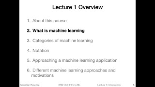 14
14
 15
15
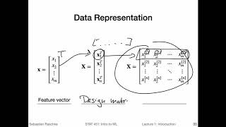 16
16
 17
17
 18
18
 19
19
 20
20
 21
21
 22
22
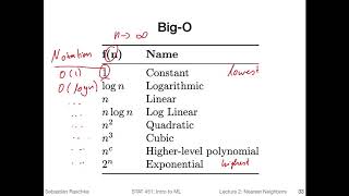 23
23
 24
24
 25
25
 26
26
 27
27
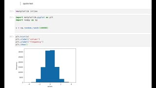 28
28
 29
29
 30
30
 31
31
 32
32
 33
33
 34
34
 35
35
 36
36
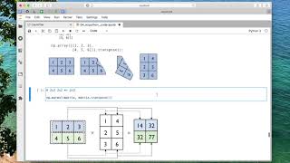 37
37
 38
38
 39
39
 40
40
 41
41
 42
42
 43
43
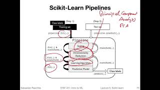 44
44
 45
45
 46
46
 47
47
 48
48
 49
49
 50
50
 51
51
 52
52
 53
53
 54
54
 55
55
 56
56
 57
57
 58
58
 59
59
 60
60

Intro to Deep Learning -- L06.5 Cloud Computing [Stat453, SS20]
Sebastian Raschka
Intro to Deep Learning -- L09 Regularization [Stat453, SS20]
Sebastian Raschka
Intro to Deep Learning -- L10 Input and Weight Normalization Part 1/2 [Stat453, SS20]
Sebastian Raschka
Intro to Deep Learning -- L10 Input and Weight Normalization Part 2/2 [Stat453, SS20]
Sebastian Raschka
Intro to Deep Learning -- L11 Common Optimization Algorithms [Stat453, SS20]
Sebastian Raschka
Intro to Deep Learning -- L12 Intro to Convolutional Neural Networks (Part 1) [Stat453, SS20]
Sebastian Raschka
Intro to Deep Learning -- L13 Intro to Convolutional Neural Networks (Part 2) 1/2 [Stat453, SS20]
Sebastian Raschka
Intro to Deep Learning -- L13 Intro to Convolutional Neural Networks (Part 2) 2/2 [Stat453, SS20]
Sebastian Raschka
Intro to Deep Learning -- L14 Intro to Recurrent Neural Networks [Stat453, SS20]
Sebastian Raschka
Intro to Deep Learning -- L15 Autoencoders [Stat453, SS20]
Sebastian Raschka
Intro to Deep Learning -- L16 Generative Adversarial Networks [Stat453, SS20]
Sebastian Raschka
Intro to Deep Learning -- Student Presentations, Day 1 [Stat453, SS20]
Sebastian Raschka
1.2 What is Machine Learning (L01: What is Machine Learning)
Sebastian Raschka
1.3 Categories of Machine Learning (L01: What is Machine Learning)
Sebastian Raschka
1.4 Notation (L01: What is Machine Learning)
Sebastian Raschka
1.1 Course overview (L01: What is Machine Learning)
Sebastian Raschka
1.5 ML application (L01: What is Machine Learning)
Sebastian Raschka
1.6 ML motivation (L01: What is Machine Learning)
Sebastian Raschka
2.1 Introduction to NN (L02: Nearest Neighbor Methods)
Sebastian Raschka
2.2 Nearest neighbor decision boundary (L02: Nearest Neighbor Methods)
Sebastian Raschka
2.3 K-nearest neighbors (L02: Nearest Neighbor Methods)
Sebastian Raschka
2.4 Big O of K-nearest neighbors (L02: Nearest Neighbor Methods)
Sebastian Raschka
2.5 Improving k-nearest neighbors (L02: Nearest Neighbor Methods)
Sebastian Raschka
2.6 K-nearest neighbors in Python (L02: Nearest Neighbor Methods)
Sebastian Raschka
3.1 (Optional) Python overview
Sebastian Raschka
3.2 (Optional) Python setup
Sebastian Raschka
3.3 (Optional) Running Python code
Sebastian Raschka
4.1 Intro to NumPy (L04: Scientific Computing in Python)
Sebastian Raschka
4.2 NumPy Array Construction and Indexing (L04: Scientific Computing in Python)
Sebastian Raschka
4.4 NumPy Broadcasting (L04: Scientific Computing in Python)
Sebastian Raschka
4.5 NumPy Advanced Indexing -- Memory Views and Copies (L04: Scientific Computing in Python)
Sebastian Raschka
4.3 NumPy Array Math and Universal Functions (L04: Scientific Computing in Python)
Sebastian Raschka
4.7 Reshaping NumPy Arrays (L04: Scientific Computing in Python)
Sebastian Raschka
4.6 NumPy Random Number Generators (L04: Scientific Computing in Python)
Sebastian Raschka
4.8 NumPy Comparison Operators and Masks (L04: Scientific Computing in Python)
Sebastian Raschka
4.9 NumPy Linear Algebra Basics (L04: Scientific Computing in Python)
Sebastian Raschka
4.10 Matplotlib (L04: Scientific Computing in Python)
Sebastian Raschka
5.1 Reading a Dataset from a Tabular Text File (L05: Machine Learning with Scikit-Learn)
Sebastian Raschka
5.2 Basic data handling (L05: Machine Learning with Scikit-Learn)
Sebastian Raschka
5.3 Object Oriented Programming & Python Classes (L05: Machine Learning with Scikit-Learn)
Sebastian Raschka
5.4 Intro to Scikit-learn (L05: Machine Learning with Scikit-Learn)
Sebastian Raschka
5.5 Scikit-learn Transformer API (L05: Machine Learning with Scikit-Learn)
Sebastian Raschka
5.6 Scikit-learn Pipelines (L05: Machine Learning with Scikit-Learn)
Sebastian Raschka
6.1 Intro to Decision Trees (L06: Decision Trees)
Sebastian Raschka
6.2 Recursive algorithms & Big-O (L06: Decision Trees)
Sebastian Raschka
6.3 Types of decision trees (L06: Decision Trees)
Sebastian Raschka
6.5 Gini & Entropy versus misclassification error (L06: Decision Trees)
Sebastian Raschka
6.6 Improvements & dealing with overfitting (L06: Decision Trees)
Sebastian Raschka
6.7 Code Example Implementing Decision Trees in Scikit-Learn (L06: Decision Trees)
Sebastian Raschka
7.1 Intro to ensemble methods (L07: Ensemble Methods)
Sebastian Raschka
7.2 Majority Voting (L07: Ensemble Methods)
Sebastian Raschka
7.3 Bagging (L07: Ensemble Methods)
Sebastian Raschka
7.4 Boosting and AdaBoost (L07: Ensemble Methods)
Sebastian Raschka
7.5 Gradient Boosting (L07: Ensemble Methods)
Sebastian Raschka
7.6 Random Forests (L07: Ensemble Methods)
Sebastian Raschka
7.7 Stacking (L07: Ensemble Methods)
Sebastian Raschka
8.1 Intro to overfitting and underfitting (L08: Model Evaluation Part 1)
Sebastian Raschka
8.2 Intuition behind bias and variance (L08: Model Evaluation Part 1)
Sebastian Raschka
8.3 Bias-Variance Decomposition of the Squared Error (L08: Model Evaluation Part 1)
Sebastian Raschka
8.4 Bias and Variance vs Overfitting and Underfitting (L08: Model Evaluation Part 1)
Sebastian Raschka
More on: Neural Network Basics
View skill →





Related Reads
📰
📰
📰
📰
I Went Back to 2012 to Build AlexNet From Scratch
Medium · Deep Learning
Detecting Rice Leaf Diseases with Deep Learning
Medium · Deep Learning
Trained a neural net to reconstruct Bad Apple in real-time.
Reddit r/deeplearning
AI/ML Under the Hood — Part 29: CNN Breaking News: Proximity Matters
Medium · Deep Learning
🎓
Tutor Explanation

 DeepCamp AI