2.4 Big O of K-nearest neighbors (L02: Nearest Neighbor Methods)

Key Takeaways

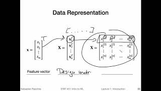
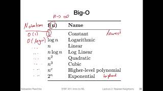
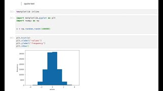
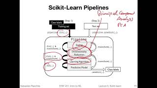
yeah now it's about time to talk about big o and k nearest neighbors run time complexity so big o is a notation or concept in computer science that is used to analyze the efficiency of algorithms so usually that refers to the runtime complexity in terms of the execution speed but then also um with a focus on how it behaves asymptotically if we have a very large data set sometimes big o notation is also used to analyze the memory efficiency so how much memory is required so if you think back of what i showed you in the very beginning of lecture two the training step of k-nearest neighbor is simply saving the training data set and that itself can be very expensive so saving the training data set can require a large amount of ram so computer memory or if we keep it on the hard drive um yeah hard drive storage space hard drive storage space space has been come has become cheaper over time but yeah depending on how we implement the k-nearest neighbor algorithm it may require that we hold all the data points in in memory and if we have a large data set let's say millions of images then this can be quite a limiting factor but right now let's more focus on a runtime complexity that means how fast k n is in the prediction step so first for those who have not heard about it let's briefly introduce big o or big o notation so here i'm just listing uh several functions that uh are used for basically describing how efficient an algorithm is so we could also maybe extend this list and call this column notation and then we have a big o of 1 of log n and so forth and we usually use these functions here to denote the the complexity or the runtime of other functions so these are the common ones that are usually used in the context of big o um i will show you a concrete example how to find out the runtime complexity of certain functions in a few moments but yeah i will also on canvas if you have not heard about big o before post some reading material and some introductory reading material about big o there's also something called big theta and big omega so they are related concepts so maybe it would not hurt to read about this in a i would say more detailed tutorial because in this class we don't focus that much on computer science it's just that we use big o here right now to understand the k nearest neighbor algorithm so in this table i'm sorting also the functions from lowest runtime complexity to highest runtime complexity so that means uh yeah the the higher up the function is on the list the better the faster it would execute for example so what we have is just to maybe briefly go over it we have a constant one so constant means no matter how big my data set is um this function would never become more expensive if n increases so we we usually look at the case where n approaches infinity so if this grows really really large let's say infinitely large how would my function behave a constant function wouldn't be affected by that at all so it would execute at the same or in the same manner and that is the ideal case scenario so functions like that that are that fast and not affected by the number of data points let's say in machine learning that would be awesome but of course it's usually not realistic logarithmic is also pretty good still linear is also still pretty good but of course not good as good as logarithmic then we have log linear growth it it's a bit slower than linear but again not bad uh where it becomes bad or what people kind of start consider as not ideal is everything let's say starting with quadratic or beyond so quadratic cubic or higher level polynomial complexity and especially exponential complexity that's usually considered very bad and in this case it's not ideal to use such algorithms for very large data sets yet to get a more visual impression of how the runtime complexity looks like as a function of n i made a plot here so on the x axis that's n the size of the data set and f of n is basically the complexity of the algorithm so basically what happens if i plug in n into into the function here so as you can see uh if we are at the very low end here around two it doesn't really matter which algorithm we use it's about the same uh runtime so we can also maybe um yeah consider this as a time that it takes to run the algorithm not just only the output of the function but really like a runtime so the higher the worse and the lower the better of course so we can see as we increase n certain functions become increasingly increasingly bad it's hard to see how well the quadratic one is doing because we are really here at a very small level still and um also we have a large scale so this scale is not really zoomed in into this area here so it's kind of hard to see how really how very expensive the quadratic already is but what we can see is that something like cubic becomes really bad really fast and then especially this um exponential one it is like exploding very soon even with small numbers so usually we want to really avoid exponential growth in machine learning in terms of the data set size so to explain a little bit more about how we get from a certain let's say function to the big o notation of that function i'm providing an example here so this is a simple function a credit quadratic function and this would basically reduce to a big o complexity of x squared so quadratic the reason is that we usually only look at the dominant term so the dominant term is the one that grows the fastest in this case it would be um this term here because uh and like we've seen in the previous slide comparison to this term the growth of this one and this one is really natural so these are so small that let's say they're so small if we go to n infinity that we can just ignore them and then also it doesn't really matter whether we have 14 times x squared or just x squared when we go um with n really large it's it'll be both really large numbers so usually we also would drop this and just focus on on the um x here so that is how we would get the big o notation of this function so let's take a look at a different function now yeah so like you saw in the previous slide scaling factors are usually dropped when we do the or when we derive the big o notation so in the for this example might be useful if you pause the video for now and um just maybe try to solve it yourself and then i will give you the solution in three seconds yes so again like in the previous slide the solution would be um or we would be focusing on the dominant terms so we would be dropping this term here and this factor here just focus on the x so we have x log and then again this is negative if we go from x or we if we consider x to be infinitely large whereas x grows infinitely large so in this case what we would have here what would remain is x log x so again yeah dropping the non-dominant terms focusing on the dominant terms here and that would be log linear growth in that case oh yeah so one additional note i wrote x log x and not x log 2 x so i have the natural logarithm instead of the logarithm with basis 2. and it's because it doesn't really matter which one we use so we um we don't really distinguish between different logarithms we usually just use the natural logarithm and yeah why is that i mean if you think about transforming the base of a logarithm for example if i go from log 2 to let's say the log of base is 10 or the block with base is 10. how i would write that is simply log 10 of x divided by log 10 should be 2 right so i could express it like as follows and then you can see if i just rewrite this as um 1 over look 10 2 times look 10 x you can see the x is inside here so here in this term there is no x really involved so it's just a scaling factor so we can just drop this scaling factor and now i have log 10 of x here so um for the big o notation but of course i can do that with any basis so i can also use the natural logarithm so i can just drop the 10 here so we have a natural logarithm now some people write the natural logarithm also as ln but in this class we will just use log for the natural logarithm which is more common so i can also do this and then the big o notation for this function here would be x log x right so in that case we don't have to worry about the basis of the logarithm you can just simply ignore that as well yeah instead of giving you another boring symbolic function i thought i would give you a python function here to explain um big o notation or just to show you an example a concrete example of applying big o notation to a computational algorithm so here i implemented matrix multiplication a function for matrix multiplication between two matrices a and b and this is a very inefficient way to do a matrix multiplication in python and i was just doing this intentionally because next lecture i'm going to show you a more efficient way of doing that the point here really is not the efficiency of this matrix multiplication it's more about just having a function so that we can look at the big o complexity or the runtime complexity of this function so let's maybe walk through this function step by step so what am i doing here so again the inputs to this function are these two matrices um a and b so i'm actually calling it here so um i'm calling the matrix function multiplication function here so the inputs are a and b the two matrices and there will be an output matrix c so c that's what's getting returned here as my output matrix so i'm just setting it up in the beginning so that we have a matrix of zeros and then we populate the matrix with the values so as you may know if we multiply two matrices and we have let's say matrix um m times p let's let's just use the concrete numbers we have a matrix a with dimensions um two times three and then the second matrix is three times two right so three rows one two oops one two three two columns so the output dimension would be output dimension would be two times two right so this would be my output dimension so i'm just setting it up here so here sorry here in this block i'm setting up my output matrix it will be then a matrix of 2 times 2 because here i'm doing this i'm iterating i'm putting a 0 for each row in length a so because i'm using a python list here the length of a is 2 because um this list has two sub lists so each row is a sublist sub list one sub is two so this will be giving me a list of two and then for each column i will um do the same thing here for each column in b so again this will evaluate to two so i will have a two by two matrix this looks a little bit complicated this is called list oops i hate it when it happens list comprehension this is called list comprehension okay so but the focus is not really here on creating the output it's um it's important but we can see that here we have two for loops whereas here we have three for loops so the majority of the time in this function will be spent will be spent here right so not in not in here so let's see how we carry out the actual matrix multiplication so what i'm doing here is for each row in my matrix a so i'm iterating first over the rows so i'm starting with the first row and then let's say for the first row which is one two three right for the first row then i'm going through the columns in b so the columns in b um these and these so now let's say we consider the first column 5 6 7 so that's where we are right now we have this first row in this first column and then i'm saying for each column in a so i'm now iterating through columns here so we are let's say still in the first iteration we're entering over columns i'm adding the existing value in c we start with the value 0 right so that would be the value 0 and then we multiply between the first column and the first value so the first column here and the first value in my um in this column here so i'm basically updating it like this right so i'm multiplying one times five and then i'm putting one times five here to update the first value so next we would uh look at the lower end or the deepest for loop to complete the deepest for loop first so which is this one so again we we said we iterate over call a which is um the position in um the column position in in this row here in the first row still and we use that call a here and here sorry here and here so we use that before to compute one times five and then update the position zero now what we do is um i should maybe say no the value here would be five after the first update now what we do is we advance one more position but again because we use it here and here we also advance this position here so we are at six now so the second update would be one times six which is six and we add this addition here we added to the previous result again so this should be updated now and should be 11 and so forth and we would yeah complete this um and then after we completed this for loop with a third number here we would um go back completing this for loop and so forth so once we've done that we would get the this this following result here and if you have not followed exactly how this python function works don't worry so much about it that's not the point of this slide the point of the slide is really the runtime complexity so we would try to um find what are the expensive parts here that depend on the input size so in this case what we have is we have three for loops so these are the expensive for loops of course we also have some for loops here but there are only two nested follow-ups so the really the expensive part is is going to happen here so if we think of matrices in this case let's say in case of quadratic matrices like a quadratic shape what we can see here is that we are iterating over the rows and over the columns and again over the columns of that row so in that case um if we consider n the number of rows and the number of columns of this matrix because there are three four loops what we would find is that the runtime complexity of this function is n cubed and as we've seen earlier in the plot n cubed that's actually a pretty expensive algorithm so in practice we would never use such an algorithm here in practice there way more efficient way to do a matrix multiplication in python yeah so now the more interesting question what is the runtime complexity of the k-nearest neighbor algorithm so if you think of the brute force search that we introduced in the beginning for the one nearest neighbor search we are searching for k near neighbors so we we want to carry out the search k times so we search for k neighbors and in the brute force search if we use the naive approach that we covered at the beginning of this lecture in the first video we are looking at each training example so we have k neighbor neighbors and we check each training example to do the distance computation and the training data set let's say we call that n we have n training examples so that depends on n so if we have 100 training examples we have to do 100 um distance computations against the query points and if we want to use k numbers if you want to find k n neighbors and we use a naive approach we have to repeat this process on k times but they are more efficient way of doing that but in the most simple case we would be k times searching for the neighbor in the n sized training set and then another factor is if you think back of the euclidean distance the distance depends on all the dimensions so if we have a euclidean distance with a sum over where all the distances between let's say some query point and some um data point in the training set so this is for one data point let's let's call this i the i training point in the data set we would have of course n times these computations so if i have the euclidean distance like that this would depend on the dimensions so if we have m dimensions we would have the distance computation depending on m the number of dimensions so if i would then consider that i would have k times n times m that's my runtime complexity of a naive application of k nearest neighbors of course um k is usually very small we usually use something like 5 or 3 5 7 10 something like that so in that case maybe you can ignore that okay here and for m i mean usually also we have very large training sets and lower dimensions so usually we have n it's much bigger than m so in that case we maybe can also drop the m here and in that case what remains is um runtime complexity of n as the size of the training set and that would be for the most naive implementation of the k nearest neighbor algorithm let us briefly think about how we can make k nearest neighbor algorithms more efficient so maybe also that's a good point here to pause the video and to brainstorm a little bit and think about possible ways for making k-nearest neighbors more efficient and maybe you can even take an hour half an hour go for a walk and think about it and come back later and continue this video it's one of the advantage of having an online video compared to in-person classes and after yeah after you've done that we will talk about some of the possible ways so i'm intentionally leaving this part this slide blank now and in the following slides i will show you again the naive k nearest neighbor implementation then i will show you one little trick and in the following video i will show you some more tricks and maybe uh if you thought about potential ways your way may be different from what other people tried and that would be then an excellent class project or maybe even research project so here is one naive way um how we can implement the k nearest neighbor search so i just call that naif sorry if nearest neighbor search um there are of course many different ways we can do that but that's on the i would say most simple one i can think of i call this variant a i will show you in a next slide another idea i had for implementing k nearest neighbors so what's going on here so first i will start with the data set dk so this is um we start with an empty data set so this will be the data set holding our k nearest neighbors and then we implement the while loop we say while the size of the set of the set decay here is smaller than k then continue doing something and that is finding a new neighbor that we can add to the set so how do we find the neighbor this is similar to what i've shown you in the very first video of lecture two so we start out by setting the closest distance to infinity and then we iterate over the training set for all the data points that we have not considered yet so for the symbol here means for all i data points that are not contained in the set decay so what i do then is i compute the current distance between my query data point that's the point i want to classify and the ith data point in the training set so the is data point is what we are entering or iterating over so we have n data points in the training set like always and then we say if the current distance is smaller than the closest distance we start with infinity then we keep that point so we consider it as a closest point so after each loop here let me use a different color after each loop over the training set we will find one neighbor that we haven't found before so by each loop we increase the size of decay until it reaches size k so what we have is we have k times a for loop over the n training data points so what would be the big o complexity of this maybe pause the video and think a little bit about this yeah i hope this was pretty straightforward so this would be k n because we look for k near neighbors in the n sized data set that's one way of implementing k nearest neighbors here i thought about a different way for implementing k nearest neighbors i call that variant b it's basically doing the same thing we did in the previous slide backwards so i start with a subset dk which is the whole training set and again while the length of the k is not equal to k we do continue doing something but instead of drawing decay like in the previous one in the previous line slide we said if dk is smaller than k now i say if dk is greater than k so what i'm doing now is i'm eliminating data points from this um set decay until i reach my desired number of neighbors so this because we eliminate we start with the largest distance setting it to 0 because we want to find the point that is the farthest away from our query point and remove that so we set the largest distance to zero and then again for each data point in the training set um but also again we only consider the ones that are not already con contained in in the subset here oh sorry in this case we are considering only the ones that are contained in the subset because this is what we want to eliminate we don't want to consider points that we already eliminated in the previous round so for all the data points in the subset i compute again the current distance so we compute the current distance if the current distance is larger than the largest distance in the first iteration this will be of course true because the largest distance will be likely larger than zero otherwise it would be exactly the query point if that's true if we find a point that is larger away than the largest distance we already have then we save that point and then we remove it from decay and we remove points until the size of decay matches k so i have a greater sign here so if this is true so if k sorry if the length of decay if we want to find let's say five neighbors and the size of dk oops size of decay is six then we would still meet this criterion here and then execute the last while loop and in the last while loop again we remove one more data point so after this while loop d k will also be size five and then we can stop so what is the time complexity of this variant b so what do you think yeah so in this case since we go backward we start with n training data points and then we eliminate right so we have n minus k and then because we have a for loop we have a for loop for each neighbor that or for each data point that we remove from our decay list so it should be times n so what would be the time complexity of this approach that would be then n minus k i should put this in parentheses times n so which one is more efficient variant a or b because that depends on the size of um k so if we have a large k uh compared to n then of course um variant b would be more efficient than a but in all likelihood n is much much larger than k so that case i would say um variant a is more efficient yeah another idea i had is using a priority queue that can help us speeding up k-nearest neighbor implementations so in the previous two slides variant a and variant b kind of suffered from the problem that we checked the training data set repeatedly which can be wasteful i think so we could for example use a priority queue um and kind of keep track of our nearest neighbors as we check the data set so we don't have to check it k times because here in the previous slide we basically selected one neighbor um when let's say variant a we selected one neighbor and then once we selected it we started all over again and did the same check over all n minus 1 data points to find the second neighbor so what we could do is we could initiate a priority queue so for example if we are interested in k equals five neighbors we could um take the first let's say or just randomly five data points in the training set and initialize a priority queue for example let's say we call it the data point x 5 x i don't know x 13 x 4 and let's let's change this to k equals 3 so i don't have to write that much um let's say we found these five uh three random points and we can keep track of them as we check our training set so when we iterate over our training set we check for each data point in the training set is it closer than this one if yes then we replace this point here with the point in the training set if no we check this one and say okay is this point closer to my query point than this given training point if yes again we swap it otherwise we move on to the next one and we say if this data point is closer to the current training point um then we swap this one with the current training data point otherwise we we continue up to the next training point so in that way um we only have one sweep through the training set we don't do the n checks multiple times right so that way um that can help us speeding up the k nearest neighbor search and yeah for this priority queue we can use a data structure also for example a heap data structure to make this more efficient and then this would eventually come down to something like um log k times n so we again have at least one time we really have to sweep over the whole training set but we don't have to do it we don't have to do a full sweep again in the next round for the k nearest neighbors so i just set um heap data structure so what is the heap data structure you don't really have to know this for this class really this is like a computer science concept a data structure in computer science i will post a link on canvas for further reading if you're interested but really you don't have to know what a you don't have to know what a heap is for this class here but no if you're interested let me just quickly tell you what a heap is so it's just a data structure for organizing a data set or an array and it allows us to find certain points more efficiently so let me uh draw a binary heap so it's kind of like a decision tree let's consider a try data set let me just pick some random numbers i don't know 1 8 6 5 9 7 so let's say i have an array like this i would organize it into a heap data structure by starting first i would basically construct the initial heap so i would go put the first element at the root and then it's a binary data structure so what i would do is i would take the second two elements put them here eight six you can put the larger one to the left for example but usually we go just how the data or array is organized then i have a five and nine so i start always on the left side i'll just put the five here the nine here and the seven the remaining one here because this is like an unorganized heap so we would then in the next step um yeah sort this array so how that works is for example i could all put all the largest values on top and for that i would do several swaps so i would for example swap these two numbers so six and the seven so after swapping them i will have the seven here and the six here um and then i can use a different color i can swap these two and in one swoop um because nine is greater than eight and eight is greater than one so i can also swap these two here so in one step how that would look like after a swap i would have the nine here the one here right and the eight here and then of course i can swap the one and the eight right so let me cancel or remove this so you can see what we currently have and then the last step i because eight is greater than one i would swap these two so in the end i would then have the one down here the eight up here so the cleaned up version of the heap would be nine eight five right here one seven six and this one allows me for example more efficiently to look up certain values more efficiency efficiently so if i want to find the largest value i would stop at a root node and then you can go through the seep basically and find the largest value always basically um to the left so large uh the larger one is to the left so here in this case the eight and then here the right side is the seven and then for each root node i have again like an organization where the larger value is to the left and the smaller value is to the right and i just see um since we're interested in similarity and distance it would actually be more useful to have a heap that is organized such that the smallest values are on top so what i was just drawing is a max heap you can also draw a min heap that would actually be more useful for nearest neighbor search with a priority queue but again this is like a detail you don't have to worry about in this class i was just briefly going over the concept over of a heap i can just post some tutorial if you're interested in learning more about it but again you don't have to really understand how a heap works so next um in the next video i will make this a separate video i will show you some more tricks for making k-nearest neighbors more efficient so the priority queue is like a nice idea but the priority queue is also not super efficient compared to some other tricks that people usually use in practice