What do neural networks learn?

Key Takeaways

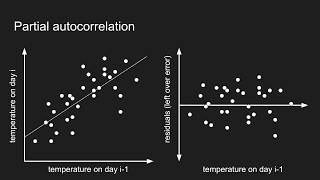
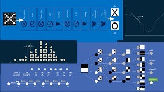
neural networks are famously difficult to interpret it's hard to know what they're actually learning when we train them so let's take a closer look and see whether we can get a good picture of what's going on inside just like every other supervised machine learning model neural networks learn relationships between input variables and output variables in fact we can even see how it's related to the most iconic model of all linear regression simple linear regression assumes the straight line relationship between an input variable X and an output variable y x is multiplied by a constant M which also happens to be the slope of the line and it's added to another constant B which happens to be where the line crosses the Y AIS we can represent this in a picture our input value X is multiplied by m our constant B is multiplied by 1 and then they get added together to get y this is a graphical representation of y = mx + b on the far left the circular symbols just indicate that the value is passed through the rectangles LEL labeled m and b indicate that whatever goes in on the left comes out multiplied by m or B on the right and the box with the capital Sigma indicates that whatever goes in on the left gets added together and spit out on the right we can change the names of all the symbols for a different representation this is still a straight line relationship we've just changed the names of all the variables the reason we're doing this is to translate our linear regression into the notation we'll use in neural networks this will help us keep track of things as we move forward at this point we have turned a straight line equation into a network a network is anything that has nodes connected by edges in this case xb0 and X sub1 are our input nodes V sub Z is an output node and our weights connecting them are edges this is not the traditional sense of a graph meaning a plot or a grid like in a graphing calculator or graph paper it's just the formal word for a network for nodes connected by edges another piece of terminology you might hear is a directed a cyclic graph abbreviated as d a or dag a directed graph is one where the edges just go in One Direction in our case input goes to Output but output never goes back to input our edges are directed a cyclic means that you can't ever draw a loop once you have visited a node there's no way to jump from edges to nodes to edges to nodes to get back to where you started everything Flows In One Direction Through the graph we can get a sense of the type of models that this network is capable of learning by choosing random values for the weights W Sub 0 0 and W sub 1 Z and then seeing what relationship pops out between x sub 1 and V Sub 0 remember that we set X Sub 0 equal to 1 and are holding it there always this is a special node called a bias node it should come as no surprise that the relationships that come out of this linear model are all straight lines after all we've taken our equation for the line and rearranged it but we haven't changed it in any substantial way there's no reason we have to limit ourselves to just one input variable we can add an additional one now here we have an X of 0 an X of 1 and an x sub 2 we draw an edge between x sub 2 and our summation with the weight w sub 2 0 x sub 2 * W sub20 is again U sub20 and all of our U's get added together to make a V subz and we could add more inputs as many as we want this is still a linear equation but instead of being two-dimensional we can make it three-dimensional or higher writing this out mathematically could get very tedious so we'll use a shortcut we'll substitute the subscript RT I for the index of the input it's the number of the input we're talking about this allows us to write U sub i0 where our U sub I equals x sub itimes W sub i0 and again our output V Sub 0 is just the summation over all values of I of U sub i0 for this three-dimensional case we can again look at the models that emerge when we randomly choose our W sub I zeros our weights as we would expect we still get the three-dimensional equivalent of a line a plane in this case and if we were to extend this to more inputs we would get the M dimensional equivalent of a line which is called an m-dimensional hyperplane so far so good now we can start to get fancier our input X sub1 looks a lot like our output V Sub 0 in fact there's nothing to prevent us from taking our output and then using it as an input to another Network just like this one now we have two separate identical layers we can add a subscript Roman numeral I and a subscript Roman numeral I I or two to our equations depending on which layer we're referring to and we just have to remember that our xub 1 in Layer Two is the same as our V sub Z in layer 1 because these equations are identical and each our layer each of our layers work just the same we can reduce this to one set of equations adding a subscript capital L to represent which layer we're talking about as we continue here we'll be assuming that all the layers are identical and to keep the equations cleaner we'll leave out the capital L but just keep in mind that if we were going to be completely correct in verbose we would add the L subscript onto the end of everything to specify the layer it belongs to now that we have two layers there's no reason that we can't connect them in more than one place instead of our first layer generating just one out output we can make several outputs in our diagram we'll add a second output V sub one and we'll connect this to a third input into our second layer xub 2 keep in mind that the X subz input to every layer will always be equal to one that bias node shows up again in every layer now there are two nodes shared by both layers we can modify our equations accordingly to specify which of the shared nodes we're talking about they behave exactly the same so we can be efficient and reuse our equation but we can specify subscript J to indicate which output we're talking about so now if I'm connecting the I input to the jth output then I and J will determine which weight is applied and which U's get added together to create the output V subj and we can do this as many times as we want we can add as many of these shared nodes as we care to the model as a whole only knows about the input x sub one into the first layer and the output V sub Z of the last layer from the the point of view of someone sitting outside the model the shared nodes between layer 1 and Layer Two are hidden they're inside the Black Box because of this they're called hidden nodes we can take this TW layer linear Network create a 100 hidden nodes set all of the weights randomly and see what model it produces even after adding all of this structure the resulting models are still straight lines in fact it doesn't matter how many layers you have or how many hidden nodes each layer has any combination of these linear elements with weights and sums will always produce a straight line result this is actually one of the traits of linear computation that makes it so easy to work with but unfortunately for us it also makes really boring models sometimes a straight line is good enough but that's not why we go to neural networks we're going to want something a little more sophistic icated in order to get more flexible models we're going to need to add some nonlinearity we'll modify our linear equation here after we calculate our output V Sub 0 we subject it to another function f which is not linear and we'll call the result y sub Z one really common nonlinear function to add here is the logistic function it's shaped like an S so sometimes it's called a sigmoid function too although that can be confusing because technically any function shaped like an S is a sigmoid we can get a sense of what logistic functions look like by choosing random weights for this one input one output one layer Network and meeting the family one notable characteristic of logistic functions is that they live between 0o and one for this reason they're also called squashing functions you can imagine taking a straight line and then squashing the edges and bending and hammering it down so that the whole thing fits between zero and one no matter how far out you go working with logistic functions brings us to another connection with machine learning models logistic regression this is a bit confusing because regression refers to finding a relationship between an input and an output usually in the form of a line or a curve or a surface of some type logistic regression is actually used as a classifier most of the time it finds a relationship between a continuous input variable and a categorical output variable it treats observations of one category as zeros treats observations of the other category as ones and then finds the logistic function that best fits all those observations then to interpret the model we add a threshold often around5 and wherever the curve crosses the threshold there's a demarcation line everything to the left of that line is predicted to fall into one category and everything to the right of that line is predicted to fall into the other this is how a regression algorithm gets modified to become a classification algorithm as with linear functions there's no reason not to add more inputs we know that logistic regression can work with many input variables and we can represent that in our graph as well here we just add one in order to keep the plot threedimensional but we could add as many as we want to see what type of functions this network can create we can choose a bunch of random values for the weights as you might have expected the functions we create are still shaped but now they're three-dimensional they look like a tablecloth laid across two tables of unequal height more importantly if you look at the contour lines projected down onto the floor of the plot you can see that they are all perfectly straight the result of this is that any threshold we choose for doing classification we'll split our input space up into two halves with the the divider being a straight line This is why logistic regression is is described as a linear classifier whatever the number of inputs you have whatever dimensional space you're working in logistic regression will always split it into two halves using a line or a plane or a hyperplane of the appropriate Dimensions another popular nonlinear function is the hyperbolic tangent it's closely related to the logistic function and can be written in a very symmetric way we can see when we choose some random weights and look at examples that hyperbolic tangent curves look just like logistic curves except that they vary between minus one and plus one just like we tried to do before with linear functions we can use the output of one layer as the input to another layer we can stack them in this way and can even add hidden nodes the same way we did before here we just show two hidden nodes in order to keep the diagram simple but you can imagine as many as you want there when we choose random weights for this network and look at the output we find that things get interesting we've left the realm of the linear because the hyperbolic tangent function is nonlinear when we add them together we get something that doesn't necessarily look like a hyperbolic tangent we get curves Wiggles Peaks and valleys and a much wider variety of behavior than we ever saw with single layer networks we can take the next step and add another layer to our Network now we have a set of hidden nodes between layer one and Layer Two and another set of hidden nodes between Layer Two and layer three again we choose random values for all the weights and look at the types of Curves it can produce again we see Wiggles and Peaks valleys and a wide selection of shapes if it's hard to tell the difference between these curves and the curves generated by a two-layer Network that's because they're mathematically identical we won't try to prove it here but there's a cool result that shows that any curve you can create learning a many using a many layer Network you can also create using a two- layer Network as long as you have enough hidden nodes the advantage of having a many layered network is that it can help you create more complex curves using fewer total nodes for instance in our two layer Network we used a 100 hidden nodes but in our three- layer Network we used 11 hidden nodes in the first layer and nine hidden nodes in the second layer that's only a fifth of the total number we used in our two- layer Network work but the curves it produces show similar richness we can use these fancy Wiggly lines to make a classifier as we did with logistic regression here we use the zero line as the cut off everywhere that our curve crosses the zero line there's a divider in every region that the curve sits above the zero line we'll call this category a and similarly everywhere the curve is below the zero line we have category B what distinguishes these nonlinear classifiers from linear ones is that they don't just split the space into two halves in this example regions of A and B are interleaved building a classifier around a multi-layer nonlinear Network gives it a lot more flexibility it can learn more complex relations this particular combination of multi-layer network with hyperbolic tangent nonlinear function has its own name a multi-layer perceptron as you can guess when you have only one layer it's just called a perceptron and in that case you don't even need to add the nonlinear function to make it work the function will still cross the xaxis at all the same places here is the full Network diagram of a multi-layer perceptron this representation is helpful because it makes every single operation explicit however it's also visually cluttered and it's difficult to work with because of this it's most often simplified to look like circles connected by lines this implies all the operations we saw in the previous diagram connecting lines each have a weight associated with them hidden nodes and output nodes perform summation and nonlinear squashing but in this diagram all of that is implied in fact our bias nodes the nodes that always have a value of one in each layer are emitted for clarity so our original Network reduces to this the bias nodes are still present and their operation hasn't changed at all but we leave them out to make a cleaner picture we only show two hidden nodes from each layer here but in practice we used quite a few more again to make the diagram as clean as possible we often don't show all the hidden nodes we just show a few and the rest are implied here's a generic diagram then for a three- layer single input single output Network notice that if we specify the number of inputs the number of outputs and the number of layers and the number of hidden nodes in each layer then we can fully Define a neural network we can also take a look at a two-input single output neural network because it has two inputs when we plot its outputs it'll be a three-dimensional curve we can once again choose random weights and generate curves to see what types of functions this neural network might be able to represent this is where it gets really fun with multiple inputs multiple layers and nonlinear activation functions neural networks can make really crazy shapes it's almost correct to say that they could make any shape you want it's worth taking a moment though to notice what its limitations are first notice that all of the functions fall between plus and minus one the dark red and the dark green regions kiss the floor and the ceiling of this range but they never cross it this neural network would not be able to fit a function that extended outside of this range also notice that these functions all tend to be smooth they have Hills and dips and valleys and wiggles and even points and Wells but it all happens relatively smoothly if we hope to fit a function with a lot of jagged jumps and drops this neural network might not be able to do a very good job of it however aside from these two limitations the variety of functions that this neural network can produce is a little mindboggling we modified a single output neural network to be a classifier when we looked at the multi-layer perceptron now there's another way to do this we can use a two output neural network instead outputs of a three- layer one input two output neural network like this we can see that there are many cases where the two curves cross and in some instances they cross in several places we can use this to make a classifier wherever the one output is greater than another it can signify that one category dominates another graphically wherever the two output functions cross we can draw a vertical line This chops up the input space into regions in each region one output is greater than the other for instance wherever the blue line is greater we can assign that to be category a then wherever the peach colored line is greater those regions are category B just like the multi-layer perceptron this lets us chop the space up in more complex ways than a linear classifier could regions of category a and category B can be shuffled together arbitrarily when you only have two outputs the advantages of doing it this way over a multi-layer perceptron with just one output are not at all clear however if you move to three or more outputs the story changes now we have three separate outputs and three separate output functions we can use our same Criterion of letting the function with the maximum value determine the category we start by chopping up the input space According to which function has the highest value each function represents one of our categories we're going to assign our first function to be category a and label every region where it's on top as category a then we can do the same with our second function and our third using this trick we are no longer limited to two categories we can create as many output nodes as we want and learn and chop up the input space into that many categories it's worth pointing out that the winning category may not be the best by very much in some cases you can see they can be very close one category will be declared the winner but the next runner up may be almost as good a fit there's no reason that we can't extend this approach to two or more inputs unfortunately it does get harder to visualize you have to imagine several of these lumpy landscape plots on top of each other and in some regions one will be greater than the others in that region that category associated with that output will be dominant to get a qualitative sense for what these regions might look like you can look at the projected Contours on the floor of these plots in the case of a multi-layer percepton these plots are all sliced at the Y equals z level that means if you look at the floor of the plot everything in any shade of green will be one category and everything in any shade of red will be the other category the first thing that jumps out about these category boundaries is how diverse they are some of them are nearly straight lines albeit with a small wiggle some of them have Wilder bends and curves and some of them chop the input space up into several disconnected regions of green and red sometimes there's a small island of green or an island of red in the middle of a sea of the other color the variety of boundaries is what makes this such a powerful classification tool the one limitation we can see looking at it this way is that the boundaries are all smoothly curved sometimes those curves are quite sharp but usually they're gentle and rounded this shows the natural preference that neural networks with hyperbolic tangent activation functions have for smooth functions and smooth boundaries the goal of this exploration was to get an intuitive sense for what types of functions and category boundaries neural networks can learn when used for regression or classification we've seen both their power and their distinct preference for smoothness we've only looked at two nonlinear activation functions logistic and hyperbolic tangent both of which are very closely related there are lots of others and some of them do a bit better at capturing sharp nonlinearities rectified linear units or or relu for instance produce surfaces and boundaries that are quite a bit sharper but my Hope was to seed your intuition with some examples of what's actually going on under the hood when you train your neural network here are the most important things to walk away with neural networks learn functions and can be used for regression some activation functions limit the output range but as long as that matches the expected range of your outputs it's not a problem second neural networks are most often used for classification they've proven pretty good at it third neural networks tend to create smooth functions when used for regression and smooth category boundaries when used for classification fourth for fully connected vanilla neural networks a two- layer Network can learn any function that a deep Network can learn however a deep Network might be able to learn it with fewer nodes fifth making sure that inputs are normalized that is they have a mean near zero and a standard deviation of less than one this helps neural networks to be more sensitive to their relationships I hope this helps you as you jump into your next project happy building