How Deep Neural Networks Work
Skills:
Neural Network Basics90%
Key Takeaways
Explains how deep neural networks work using a simple example of a four-pixel camera
Full Transcript
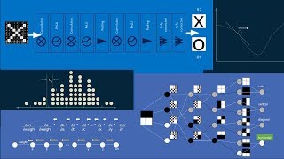
neural networks are good for learning lots of different types of patterns to give an example of how this would work uh imagine you had a four pixel camera so not not four megapixels but just four pixels and it was only black and white and you wanted to go around and take pictures of things and determine automatically then whether these pictures were of a solid all white or all dark image vertical line line or a diagonal line or a horizontal line This is tricky because you can't do this with simple rules about the brightness of the pixels both of these are horizontal lines but if you tried to make a rule about which P pixel was bright and which was dark you wouldn't be able to do it so to do this with the neural network you start by taking all of your inputs in this case are four pixels and you break them out to input neurons and you assign a number to each of these depending on the brightness or darkness of the pixel plus one is all the way white minus one is all the way black and then gray is zero right in the middle so these values once you have them broken out and listed like this on the input neurons it's also called the input vector or array it's just a list of numbers that represents your inputs right now it's a useful notion to think about the receptive field of a neuron all this means is what set of inputs makes the value of this neuron as high as it could possibly be for input neurons this is pretty easy each one is associated with just one pixel and when that pixel is all the way white the value of that in neuron is as high as it can go the black and white checkered areas show pixels that an input neuron doesn't care about if they're all the way white or all the way black it still doesn't affect the value of that input neuron at all now to build a neural network we create a neuron the first thing this does is it adds up all of the values of the input neurons so in this case if we add up all of those values we get a 0 five now to complicate things just a little bit each of the connections are weighted meaning they're multiplied by a number that number can be one or minus one or anything in between so for instance if something has a weight of minus one it's multiplied and you get the negative of it and that's added in if something has a weight of zero then it's effec ly ignored so here's what those weighted connections might look like and you'll notice that after the values of the input neurons are weighted and added the value is the final value is completely different graphically it's convenient to represent these weights as white links being positive weights black links being negative weights and the thickness of the line is roughly proportional to the magnitude of the weight then after you add the weighted input neurons uh they get squashed and I'll show you what that means you have a sigmoid squashing function sigmoid just means s-shaped and what this does is you put a value in let's say 0. five and you run a vertical line up to your sigmoid and then a horiz horizontal line over from where it crosses and then where that hits the Y AIS that's the output of your function so in this case slightly less than 0.5 it's pretty close as your input number gets larger your output number also gets larger but more slowly and eventually no matter how big the number you put in the answer is always uh less than one similarly when you go negative the answer is is always greater than negative one so this ensures that that neuron's value never gets outside of the range of plus one to minus one which is helpful for keeping the computations in the neural network bounded and stable so after you sum the weighted values of the neurons and squash the result you get the output in this case 746 that is a neuron so we can call this we can collapse all that down and this is a neuron that does a weighted sum and squash the result and now instead of just one of those assume you have a whole bunch there are four shown here but uh there could be 400 or 4 million now to keep our picture clear we'll assume for now that the weights are either plus one white lines minus one black lines or zero in which case they're missing entirely but in actuality all of these neurons that we created are each attached to all of the input neurons and they all have some weight between minus one and plus one when we create this first layer of our neural network uh the receptive Fields get more complex for instance here each of those end up combining two of our input neurons and so the value the receptive field uh the pixel values that make that first layer neuron as large as it can possibly be look now like pairs of pixels either all white or a mixture of white and black depending on the weights so for instance this neuron here is attached to this input pixel which is upper left and this input pixel which is lower left and both of those weights are positive so it combines the two of those and that's its receptive field the receptive field of this one plus the receptive field of this one however if we look at this neuron it combines our this pixel upper right and this pixel lower right it has a weight of minus one for the lower right pixel so that means it's most active when this pixel is black so here is its receptive field now uh the because we were careful of how we created that first layer its values look a lot like input values and uh we can turn right around and create another layer on top of it the exact same way with the output of one lay layer being the input to the next layer and we can repeat this uh three times or seven times or 700 times for additional layers each time the receptive Fields get even more complex so you can see here using the same logic now they cover all of the pixels and more uh more special arrangement of which are black and which are white um we can create another layer uh again all of these neurons in one layer are connected to all of the neurons in the previous layer but we're assuming here that most of those weights are zero and not shown it's not generally the case um so just to mix things up we'll create a new layer but if you notice our squashing function isn't there anymore we have something new called a rectified linear unit this is another popular neuron type so you do your weighted sum of all your inputs and instead of squashing you uh do rectified linear units uh you Rectify it so if it is negative you make the value zero if it's positive you keep the value this is obviously very easy to compute and it turns out to have very nice stability properties for neural networks as well in practice so after we do this uh because some of our weights are positive and some are negative connecting to those rectified linear units we get receptive fields and their opposites you look at the patterns there and then finally when we've created as many layers with as many neurons as we want we create an output layer here we have four outputs that we're interested in is the image solid vertical diagonal or horizontal so to walk through an example here of how this would work let's say we start with this input image shown on the left dark pixels on top white on the bottom as we propagate that to our input layer this is what those values would look like the top pixels the bottom pixels as we move that to our first layer we can see the combination of a dark pixel and a light pixel summed together get us zero gray um whereas down here we have the combination of a dark pixel plus a light pixel with a negative weight so that gets us a value of negative one there which makes sense because if we look at the receptive field here upper left pixel white lower left pixel black it's the exact opposite of the input that we're getting and so we would expect its value to be as low as possible minus one as we move to the next layer we see the same types of things combining zeros to get zeros um combining a negative and a negative with a negative weight which makes a positive to get a zero and here we have combining two negatives to get a negative so again you'll notice the receptive field of this is exactly the inverse of our input so it makes sense that its weight would be negative or its value would be negative and we move to the next layer all of these of course these zeros propagate forward um here this is a negative has a negative value and it gets has a positive weight so it just moves straight forward because we have a rectified linear unit negative values become zero so now it is zero again two but this one gets rectified and becomes positive negative times the negative is positive and so when we finally get to the output we can see they're all zero except for this horizontal which is positive and that's the answer our neural network said this is an image of a horizontal line now neural network usually aren't that good not that clean so there's a notion of with an input what is truth in this case the truth is this has a zero for all of these values but a one for horizontal it's not solid it's not vertical it's not diagonal yes it is horizontal an arbitrary neural network will give answers that are not exactly truth they might be off by a little or a lot and then the error is the magnitude of the difference between the truth and the answer given and you can add all these up to get the total error for the neural network so the idea the whole idea with learning and training is to adjust the weights to make the error as low as possible so the way this is done is we put an image in we calculate the error at the end then we look for how to adjust those weights higher or lower to either make that error go up or down and we of course adjust the weights in the way then make the error go down now the problem with doing this is each time we go back and calculate the error we have to multiply all of those weights by all of the neuron values at each layer and we have to do that again and again once for each weight um this takes forever in Computing terms uh on Computing scale and so it's not a practical way to train a big neural network you can imagine instead of just rolling down to the bottom of a simple Valley we have a very high dimensional Valley and we have to find our way down and because there are so many dimensions one for each of these weights that the computation just becomes prohibitively expensive luckily there was an inside that lets us do this in a very reasonable time and that's that if we're careful about how we design our neural network we can calculate the slope directly the gradient we can figure out the direction that we need to adjust the weight without going all the way back through our neural network and recalculating so uh just review the slope that we're talking about is when we make a change in weight the error will change a little bit and that relation of the change in weight to the change in error is the slope mathematically there are several ways to write this um we'll favor the one on the bottom it's technically most correct um we'll call it DW for shorthand every time you see it just think the change in error when I change a weight or the change in the thing on the top when I change the thing on the the bottom um this is uh does get into a little bit of calculus we do take derivatives uh that's how we calculate slope if it's new to you I strongly recommend a good semester of calculus just because the concepts are so Universal and uh a lot of them have very nice physical interpretations which I find very appealing but don't worry otherwise just gloss over this and pay attention to the rest and you'll get a general sense for how this works so in this case if we change the weight by plus one the error changes by minus two which gives us a slope of minus 2 that tells us the direction that we should adjust our weight and how much we should adjust it to bring the error down now to do this you have to know what your error function is so assume we had a error function that was the square of the weight and you can see that our weight is right at minus one so the first thing we do is we take the derivative change in error divided by change in weight D DW the derivative of weight squared is two times the weight and so we plug in our weight of minus one and we get a slope D DW of minus 2 now the other trick that lets us do this with deep neural networks is chaining and to show you how this works imagine a very simple trivial neural network with just one hidden layer one input layer one output layer and one weight connecting each of them so it's obvious to see that the value Y is just the value x times the weight connecting them W1 so if we change W1 a little bit we just take the derivative of y with respect to W1 and we get X the slope is X if I change W1 by a little bit then y y will change by x times the size of that adjustment similarly for the next step we can see that e is just the value y times the weight W2 and so when we calculate D Dy it's just W2 because this network is so simple we can calculate from one end to the other x * W1 * W2 is the error E and so if we want to calculate how much will the error change if I change W1 we just take the derivative of that with respect to W1 and get x * W2 so this illustrates you can see here now that what we just calculated is actually the product of our first derivative that we took uh the the Dy dw1 times the derivative for the next step Dy multiplied together this is chaining you can calculate the slope of each tiny step and then multiply all of those together to get the slope of the full chain derivative of the full chain so in a deeper neural network what this would look like is if I want to know how much the error will change if I adjust a weight that's deep in the network I just calculate the derivative of each tiny little step all the way back to the weight that I'm trying to calculate and then multiply them all together this computationally is many many times cheaper than what we had to do before of recalculating the error for the whole neural network for every weight now in the neural network that we've created there are several types of back propagation we have to do there's several operations we have to do for each one of those we have to be able to calculate the slope so for the first one is just a weighted connection between two neurons A and B so let's assume we know the change in error with respect to B we want to know the change in error with respect to a to get there we need to know DB da so to get that we just write the relationship between b and a take the derivative of B with respect to a we get the weight w and now we know how to make that step we know how to do that little nugget of back propagation another element that we've seen is sums all of our neurons sum up a lot of inputs to take this bra back propagation step we do the same thing we write our expression and then we take the derivative of our end point Z with respect to our step that we're uh propagating to a and DZ da in this case is just one which makes sense if we have a sum of a whole bunch of elements we increase one of those Elements by one we expect the sum to increase by one that's the definition of a slope of one one to one relation there um another element that we have that we need to be able to back propagate is the sigmoid function so this one's a little bit more interesting mathematically we'll just write it shorthand like this the sigma function um it is entirely feasible to uh go through and take the derivative of this analytically and um calculate it it just so happens that this function has a nice property that to get its derivative you just multiply it by one minus itself so this is very straightforward to calculate um another element that we've used is the rectified linear unit again to figure out how to back propagate this we just write out the relation B is equal to a if a is positive otherwise it's zero and piecewise for each of those we take the derivative so dbda is either one if a is positive or zero and so with all of these little back propagation steps and the ability to chain them together we can calculate the effect of adjusting any given weight on the error for any given input and so to train then we start with a fully connected Network we don't know what any of these weights should be um and so we assign them all random values we create a completely arbitrary random neural network we put in an input that we know the answer to we know whether it's solid vertical diagonal or horizontal so we know what truth should be and so we can calculate the error then we run it through calculate the error and using back propagation go through and adjust all of those weights a tiny bit in the right direction and then we do that again with another input and again with another input for if we can get get away with it uh many thousands or even millions of times and eventually all of those weights will gravitate they'll roll down that many-dimensional Valley to a nice low spot in the bottom where it performs really well and does pretty close to truth on most of the images if we're really lucky it'll look like what we started with with intuitively um understandable uh receptive fields for those neurons and a relatively sparse representation meaning that most of the weights are small or close to zero and it doesn't always turn out that way but what we are guaranteed is that it'll find a pretty good representation of you know the best that it can do adjusting those weights to get as close as possible to the right answer for all of the inputs so what we've covered is just a very basic introduction to the principles behind neural networks I haven't told you quite enough to be able to go out and build one of your own but if you're feeling motivated to do so I highly encourage it here are a few resources that you'll find useful you'll want to go and learn about bias neurons Dropout is a useful training tool there are several resources available from Andre karpathy who is an expert in neural networks and great at teaching about it also there's a fantastic article called the black magic of deep learning that just has a bunch of practical From The Trenches tips on how to get them working well if you found this useful I highly encourage you to visit my blog and check out several other how it works style posts and the links for these slides you can get as well to uh to use however you like there's also a link to them down in the comment section thanks for listening
Original Description
Part of the End-to-End Machine Learning School Course 193, How Neural Networks Work at https://e2eml.school/193
Visit the blog:
https://brohrer.github.io/how_neural_networks_work.html
Get the slides:
https://docs.google.com/presentation/d/1AAEFCgC0Ja7QEl3-wmuvIizbvaE-aQRksc7-W8LR2GY/edit?usp=sharing
Errata
3:40 - I presented a hyperbolic tangent function and labeled it a sigmoid. While it is S-shaped (the literal meaning of "sigmoid") the term is generally used as a synonym for the logistic function. The label is misleading. It should read "hyperbolic tangent".
7:10 - The two connections leading to the bottom most node in the most recently added layer are shown as black when they should be white. This is corrected in 10:10.
Watch on YouTube ↗
(saves to browser)
Sign in to unlock AI tutor explanation · ⚡30
Playlist
Uploads from Brandon Rohrer · Brandon Rohrer · 24 of 60
1
 2
2
 3
3
 4
4
 5
5
 6
6
 7
7
 8
8
 9
9
 10
10
 11
11
 12
12
 13
13
 14
14
 15
15
 16
16
 17
17
 18
18
 19
19
 20
20
 21
21
 22
22
 23
23
 ▶
▶
 25
25
 26
26
 27
27
 28
28
 29
29
 30
30
 31
31
 32
32
 33
33
 34
34
 35
35
 36
36
 37
37
 38
38
 39
39
 40
40
 41
41
 42
42
 43
43
 44
44
 45
45
 46
46
 47
47
 48
48
 49
49
 50
50
 51
51
 52
52
 53
53
 54
54
 55
55
 56
56
 57
57
 58
58
 59
59
 60
60

Robot Learning with a Biologically-Inspired Brain (BECCA)
Brandon Rohrer
BECCA talk at AGI 2011
Brandon Rohrer
Robot Learning with a Biologically-Inspired Brain (BECCA), The Sequel
Brandon Rohrer
BECCA listens to The Hobbit
Brandon Rohrer
Learning the building blocks of speech: BECCA extracts a hierarchy of audio features
Brandon Rohrer
BECCA listens for sound effects in The Hobbit
Brandon Rohrer
BECCA finds movie trailers while watching the Big Bang Theory
Brandon Rohrer
Listening for unexpected sounds: BECCA detects anomalies in audio data
Brandon Rohrer
Learning the building blocks of vision: BECCA extracts a spatio-temporal hierarchy of features
Brandon Rohrer
Watching for the unexpected: BECCA detects anomalies in video data
Brandon Rohrer
BECCA finds a stationary target
Brandon Rohrer
BECCA finds a stationary target at 3X speed
Brandon Rohrer
BECCA watches the X-men and Bruce Lee
Brandon Rohrer
BECCA plays Quidditch
Brandon Rohrer
BECCA chases a ball
Brandon Rohrer
BECCA chases a ball, part 2
Brandon Rohrer
Becca chases a ball, part 3
Brandon Rohrer
BECCA creates features from MNIST
Brandon Rohrer
How reinforcement learning works in Becca 7
Brandon Rohrer
Deep Learning Demystified
Brandon Rohrer
How Data Science Works
Brandon Rohrer
How Convolutional Neural Networks work
Brandon Rohrer
How Bayes Theorem works
Brandon Rohrer
How Deep Neural Networks Work
Brandon Rohrer
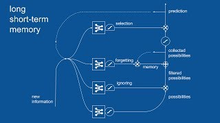
Recurrent Neural Networks (RNN) and Long Short-Term Memory (LSTM)
Brandon Rohrer
How Support Vector Machines work / How to open a black box
Brandon Rohrer
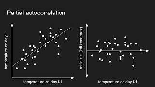
How autocorrelation works
Brandon Rohrer
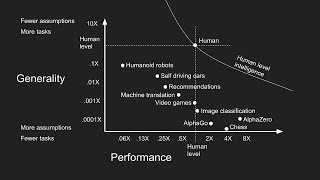
Getting closer to human intelligence through robotics
Brandon Rohrer
A minimalist's guide to slicing and indexing pandas DataFrames
Brandon Rohrer
How decision trees work
Brandon Rohrer
Data scientist archetypes
Brandon Rohrer
How to use python's datetime package
Brandon Rohrer
How optimization for machine learning works, part 1
Brandon Rohrer
How optimization for machine learning works, part 2
Brandon Rohrer
How optimization for machine learning works, part 3
Brandon Rohrer
How optimization for machine learning works, part 4
Brandon Rohrer
How convolutional neural networks work, in depth
Brandon Rohrer
How to pick a machine learning model 4: Splitting the data
Brandon Rohrer
How to pick a machine learning model 3: Choosing a loss function
Brandon Rohrer
How to pick a machine learning model 2: Separating signal from noise
Brandon Rohrer
How to pick a machine learning model 1: Choosing between models
Brandon Rohrer
How to pick a machine learning model 5: Navigating assumptions
Brandon Rohrer
What do neural networks learn?
Brandon Rohrer
Interview with iRobot's Director of Data Science Angela Bassa
Brandon Rohrer
How Backpropagation Works
Brandon Rohrer
Evolutionary Powell's method: A discrete optimizer for hyperparameter optimization
Brandon Rohrer
1D convolution for neural networks, part 1: Sliding dot product
Brandon Rohrer
1D convolution for neural networks, part 2: Convolution copies the kernel
Brandon Rohrer
1D convolution for neural networks, part 3: Sliding dot product equations longhand
Brandon Rohrer
1D convolution for neural networks, part 4: Convolution equation
Brandon Rohrer
1D convolution for neural networks, part 5: Backpropagation
Brandon Rohrer
1D convolution for neural networks, part 6: Input gradient
Brandon Rohrer
1D convolution for neural networks, part 7: Weight gradient
Brandon Rohrer
1D convolution for neural networks, part 8: Padding
Brandon Rohrer
1D convolution for neural networks, part 9: Stride
Brandon Rohrer
The Four Grand Challenges of Robots in the Home
Brandon Rohrer
How Convolution Works
Brandon Rohrer
The Softmax neural network layer
Brandon Rohrer
Batch normalization
Brandon Rohrer
Getting ready to learn Python, Mac edition #1: Files and directories
Brandon Rohrer
More on: Neural Network Basics
View skill →


Related AI Lessons
⚡
⚡
⚡
⚡
Beyond the Elephant: On Manifolds, Projections, and the Hidden Assumptions of Neural Geometry
Medium · AI
Beyond the Elephant: On Manifolds, Projections, and the Hidden Assumptions of Neural Geometry
Medium · Data Science
Beyond the Elephant: On Manifolds, Projections, and the Hidden Assumptions of Neural Geometry
Medium · Deep Learning
Beyond the Elephant: On Manifolds, Projections, and the Hidden Assumptions of Neural Geometry
Medium · LLM
🎓
Tutor Explanation