How optimization for machine learning works, part 4

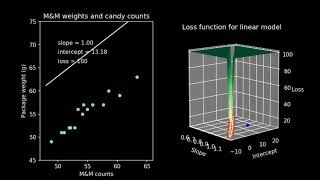
now that we've laid all the groundwork we can take things up a level and see how to apply optimization in a three parameter model by looking at another M&M data set we noticed when fitting our line that not every bag had identical M&M weights some of them were noticeably higher and some noticeably lower than others we suspect there might be an underlying pattern here and our suspicions are further aroused when we talk to some of our friends that work at the M&M factory we learned that they upgraded their equipment during the period that our M&Ms were being sampled from but we don't know exactly when if there was a change in M&M weight due to the change in equipment we would expect to see a jump at some point with the M&Ms coming after the jump having a consistently higher or lower weight when we plot the average M&M weight in the package against the manufacturing date of that package we see that there probably is a small difference there are three questions the Steven could help us answer what was the typical M&M weight before the change what was the typical M&M weight after the change and when did the change occur there are lots of generic models available these are models like linear regression or decision trees that don't know anything about where our data came from what it means or how we got it in this example we can do a little bit better than these naive models we have some extra information that helps us to make a better guess at what our model should look like given what we know it's reasonable to hypothesize a model with a constant M&M weight before and after the equipment change and a step change between them this is a three parameter model there's three numbers we need to define it completely the weight before the change the weight after and the date of the change for consistency we'll keep our loss function as the square of the deviation between our model and the day we can now perform an exhaustive search again over all possible combinations of all plausible parameter values but notice that it's taking a lot longer to compute with each additional parameter and we can get a four dimensional loss function plotting a three dimensional function is tricky but plotting a four dimensional function is really hard but we'll give it a try one trick we can use is to choose a specific value for one of our parameters what's left is a three dimensional loss function this lets us experiment and get a feel for how those two parameters interact where the sweet spot is for both of them and then we can see at least for this value of the third parameter what combination of the other two parameters produces the lowest loss in our case we have fixed the day on which the equipment was swapped out and are varying the other two parameters the weight of an M&M before the change and the weight of an M&M after the loss function helps us see what the best estimates are for these at least if we assume this particular equipment shipped today another trick we can use is to take the parameter that we chose a fixed value for our shift day and increment it just a little bit we can do this again and again and get a series of three dimensional plots what this does is to take one of our dimensions and spread it out across time we can use time to represent our fourth dimension if you look very carefully as the shift day progresses through its values you can see the bottom of our bowls jump up and down this shows how the lowest possible value for the loss function changes depending on the ship today we're looking for the very lowest of all possible values that is the optimal estimate it depends not only on our estimate of mmm weight before and after the shift day but also on our choice of the shift today there are three separate choices we have to make three separate dials we have to spin to find the best answer if you watch the bottom of the bowl very carefully as the shift day progresses you can see that it reaches a low point then jumps back up again then reaches another low point this means the gradient descent will give us different answers depending on where we start the answer is sensitive to our initial guess this is an example of non convex loss function as we mentioned before there are a few ways to handle this we won't go into them in detail here but one method that's good to have in your bag of tricks is this scattershot approach that involves choosing several random starting points and running gradient descent from each of them once you discover that several of them are ending up in the same place or the several of them are giving the same minimum value then you can be reasonably confident that you have a good answer the more random starting points you pick and the more times you choose a random starting point and try again the better your chances of finding the global optimum although you'll never be able to guarantee that you have the absolute best answer it's worth keeping in mind however that in machine learning applications we are dealing with data that's assumed to have some noise on it and then we will be applying our model to future data points that will have their own unique patterns of noise in them it's not worth our time to worry about getting the exact perfect global optimum for our purposes getting an answer that is just as good as we can get is usually good enough this one concept of looking for the lowest point in an error function is all you need to survive an optimization per machine learning it takes a lot of different forms can extend to many more parameters it can be used with generic models like logistic regression where there are just a few parameter so are a few dozen of them it can be used with very domain-specific models such as macroeconomics or agriculture the optimization method doesn't know the difference in either case all it does is tries to find the right combination of values for getting the lowest loss optimization is also at the heart of deep neural networks of success it's how all of the weights making all of the between layer connections from node to node are chosen in these models there can be thousands or even millions of parameters the loss function is not only impossible to draw on the sheet of paper it's mind-boggling to even contemplate but the math behind optimization carries on anyway doing its thing and seeking out the lowest points of the loss function that it can find a quirky thing about optimization in deep neural networks is that the loss function is known to have many dips like a many dimensional egg crate mattress depending on where you drop a marble it will very likely land in a different divot every time deep neural networks can take a long time to Train and in practice they're often trained only once starting from a single random set of initial weights that means that of all the millions of low points available on the loss function we are only going to find one this may be one of the reasons that training neural networks is such an art it's not quite as bleak as it sounds however some recent research suggests that most of these divots have the same depth like an actual egg crate mattress at least for certain types of neural networks so maybe the multitude of local minima is not as much of an issue as it might appear at first glance another part to the art of deep neural networks is the alphabet soup of gradient descent methods as you read about it you'll hear names like SGD stochastic gradient descent and AG Nesterov accelerated gradient Adam or ADA grad all of these are embellishments of gradient descent they differ in the fine details about exactly how far to step and in precisely which direction some work a little better for some problems than others but mostly they just change how fast the neural network converges to the final answer in every case the underlying goal is the same starting from a random place in a many dimensional landscape of hills and valleys find the lowest point in the nearest valley going downhill the other type of optimization that occurs in deep neural networks is hyper parameter tuning this is still just optimization but instead of optimizing the many parameters in the model it's actually optimizing the values of some of the high-level settings that determine how the model works in some cases determining how gradient descent is performed if decorating a house you can think of model training as optimization where you're choosing exactly where within a room the couch in the bookshelf and the picture should be and how they should be oriented hyper parameter tuning is the next level up it's deciding which room they should even be in to start with because testing a new set of hyper parameter values requires retraining the model entirely from scratch it takes a long time and usually a lot of computer's computational intensity has driven creative machine learning practitioners to find ways to try as few hyper parameter combinations as possible however the underlying goal and the underlying problem are still the same find the combination of values that gives the lowest loss get to the bottom of the deepest Valley you can find great job sticking in there to the end thanks for hanging in there with me I hope the concept of optimization is a little bit less scary now and then you have an intuitive sense of what's going on under the hood when the machine learning algorithms being trained good luck on building your next project