How decision trees work

Key Takeaways

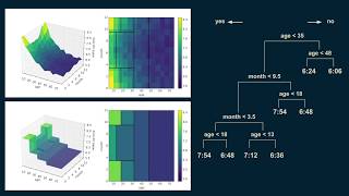
hi this is Brandon roar with how decision trees work decision trees are one of my favorite models they're simple and they're powerful in fact most high-performing Kaggle entries are a combination of XG boost which is a variant of decision tree and some very clever feature engineering the concept behind decision trees is refreshingly straightforward imagine creating a dataset by recording the time you left your house and noting whether you arrived at work on time looking at it you can see that for the most part departure times before 8:15 result in punctuality and departure times after 8:15 result in tardiness you can summarize this pattern in a decision tree the very first branching point is the question did departure occur before 8:15 there are two branches a yes and a no for consistency will keep all of our yeses on the Left placing this decision boundary divides the data up into two groups and all of all though there are some stragglers and exceptions the overall pattern is captured by placing this decision boundary at 8:15 if you depart before at 8:15 you can be reasonably sure of getting to work on time if you depart after 8:15 you can be reasonably sure of being late this is the simplest decision tree possible a single branch we can refine our estimate of punctuality by subdividing both the before 8:15 and the after 8:15 branches if we add additional decision boundaries at 8 o'clock and 8:30 then we can divide up our arrival estimate more fully those before 8 o'clock are confidently on-time those between 8 and 8:15 are probably on time but not guaranteed to be so similarly departure times after 8:15 can be divided into those after 8:30 which are almost certainly late and those before 8:30 which still have a small chance of being on time this decision tree has two levels decision trees can have as many levels as you want most often each decision point or node has only two branches this example has a single predictor variable and a categorical target variable the predictor variable is our departure time and our target variable is our punctuality whether or not we're late because it has only two distinct values its categorical decision trees with categorical targets are also called classification trees we can extend this example to the case where there are two predictor variables consider both the departure time and the day of the week we'll start counting at Monday equals one so Saturday equals six and Sunday equals seven inspecting the data we can see that on Saturday and Sunday the green filled Donuts representing being late extend further to the left this means that leaving at 8:10 is probably sufficient to get you to work on time on a weekday but probably not on the weekend to represent this in a decision tree we can start as we did before by putting a decision boundary at 8:15 any departure times after 8:15 are likely to be late departure times before 8:15 are inconsistent before we assumed that they would be on time but now we can see in the data that that's not entirely true to make our estimate better for the weekends we can subdivide the before 8:15 departure times into weekday and weekend now a weekday departure before 8:15 is confident lian time however weekend departures before 8:15 are mostly on time but not entirely we have updated the decision tree with a node that reflects this new decision boundary now we can further refine our estimate by de subdividing our weekend pre 8:15 departure times into before and after 8 o'clock before 8 o'clock almost all of the arrivals are on time between 8:00 and 8:15 the majority of them are late now we have our two-dimensional decision tree neatly divided into four regions two of them reflect on time arrivals and two of them show late arrivals this is a three level decision tree now note that not all the branches need to extend down to the same number of levels now we can look at an example with a continuous target variable rather than a categorical one when a model is used to make predictions about continuous numerical variables it's also called a regression tree so far we have looked at 1 & 2 dimensional classification trees now we'll look at regression trees let's consider the question of what time someone wakes up as predicted by their age the root of our regression tree is an estimate for the entire data set in this case if you had to make an estimate without knowing someone's age a reasonable guess would be 625 this is the root of the decision tree a reasonable first split is at age 25 on average people younger than 25 wake up at 7:05 and people older than 25 wake up at 6 o'clock there's still a lot of variation in the younger group so we can split it again now the people younger than 12 can be estimated to wake up at 7:45 and people between 12 and 25 can be estimated to wake up at 6:40 the over 25 group can be meaningfully subdivided to those between 25 and 40 wake up on average six-ten and those between 40 and 70 wake up on average at 5:50 there's still a lot of variation in the youngest group so we can further subdivided by slicing again on h8 we can refine the estimates to more closely fit the data we can also subdivide the 40 to 70 group on the 58-year line notice that we're getting to where we only have one or two data points per leaf of our tree this is a dangerous condition and can lead to overfitting which we'll talk more about in a minute the resulting tree lets us make a numerical estimate depending on someone's age if I need to estimate the wakeup time for a 36 year old for instance I can start at the top of the tree are they younger than 25 no go to the right are they younger than 40 yes go to the left the estimate then becomes 610 a.m. the structure of the decision tree lets you sort people of any age into their respective bin and make an estimate about their wakeup time we can also extend this regression tree example to have two predictor variables if we consider not only someone's age but the month of the year as well then we can find even richer patterns in North America days are longer in summer months and it gets lighter earlier in the morning in this completely unrealistic example children and teens are unburdened by the rigorous schedules of work in school and have their wakeup time driven by when the Sun comes up on the other hand adults fall into more regular patterns fluctuating only slightly with the seasons again older people in this example tend to wake up a little earlier we construct this decision tree much the same as the last one we start with the root a single estimate that roughly fits the entire data set 6:30 then we look for a good place to put a decision boundary we split the data on age 35 creating two halves one for our under 35 population with a wake-up time of 706 and one for our over 35 population with a wake-up time of 612 we repeat the process subdividing our younger population on whether it is before or after the middle of September and whether it is before or after the middle of March this isolates the winter months from the summer months winter months have a wake-up time of 7:30 for those under 35 and in the summer months at 6:56 then we can revisit our over 35 population and split them again on age 48 to get a more accurate representation we can also go back and subdivide our under 35 winter wake-up times on age 18 someone under 18 in the winter will wake up at 7 54 as opposed to 6 48 for those over 18 you can start to see the emergence of the tall corner Peaks as we make each additional cut the shape of our decision tree becomes a little bit closer to that of the original data also you'll notice in the upper right-hand plot that the decision boundaries begin to slice the data set into regions of approximately uniform color the next cut continues this trend focusing on dividing those younger than 35 in summer months to those older and younger than 13 the shape of the model becomes even more similar to that at the data you can imagine continuing this process until the model closely represents the smooth trend underlying the data each decision region would become progressively smaller the approximation to the underlying function in the data would become progressively better the power of decision trees is not without pitfalls an important one to watch out for is overfitting returning to our example of a single variable regression tree age versus wake-up time imagine that we continue to make cuts on the age axis until there were only one or two data points in each bucket when we get to this point the decision tree explains and fits the data very well it fits too well not only does it capture the underlying trend the smooth curve that the data follows but it also catches the noise the unmodeled variation that's included in the measured data if we were to take this model and use it to make predictions about new data the noise from the training data would actually make our predictions less accurate ideally we want a decision tree to capture the underlying trend but not to capture the noise one way to safeguard against this is to make sure that there are more than a handful of data points in each leaf of our decision tree that way if any noise we'll be able to average itself out another thing to watch out for is having lots of variables we started with the one-dimensional regression tree then included month data to create a two-dimensional regression tree decision trees don't care how many dimensions we have we could for instance also add latitude the amount of exercise someone gets on a given day their body mass index and any other variables that we think might be relevant to visualize this we'll use a trick shared by Geoffrey Hinton a renowned deep neural network researcher he recommends to deal with hyper planes in a 14 dimensional space visualize a 3d space and say 14 to yourself very loudly the challenge when working with many variables then becomes deciding which variable to branch on when growing our decision tree if there are very many variables then this can require a lot of computation also the more variables we add the more data we need to reliably choose between them it's easy to get into a position where the number of data points is comparable to the number of variables when our dataset is represented as a table this manifests itself as the number of rows being comparable to the number of columns there are methods for dealing with this such as randomly selecting a variable to divide on at each branch but it's something to keep an eye out for and handle mindfully as long as you keep your eyes open for places where decision trees might fail you're free to take advantage of their strengths decision trees are fantastic for when you want to make as few assumptions about your data as possible they're quite general they can find nonlinear relationships between your predictor variables and your target variable as well as nonlinear interactions between predictor variables quadratic exponential cyclical and any other relationships can all be revealed as long as you have enough data to support all the necessary cuts decision trees can also find non smooth behaviors sudden jumps and Peaks that other models like linear regression or artificial neural networks can hide sometimes there's a good reason that decision trees consistently outperform other methods on data rich problems thanks for tuning in and I hope this is helpful in building your next project