StatQuest: t-SNE, Clearly Explained
Skills:
ML Maths Basics80%
Key Takeaways
This video teaches t-SNE method for dimensionality reduction in R
Full Transcript
I'm drawing a graph. Doesn't it look cool? But I didn't know how it worked until I watched StatQuest. Hello and welcome to StatQuest. StatQuest is brought to you by the friendly folks in the genetics department at the University of North Carolina at Chapel Hill. Today we're going to be talking about t-SNE or t-SNE. To be honest, I don't actually know how it's pronounced, but it's going to be clearly explained. I know that bit. Also, this StatQuest is by request. A couple of people put it in the comments below and I got a couple of emails from other people. So I'm doing it because you guys want it. Here it goes. If you're watching this StatQuest, chances are you've seen an example of a t-SNE graph before. What t-SNE does is it takes a high-dimensional data set and reduces it to a low-dimensional graph that retains a lot of the original information. If you're not familiar with those terms of taking a high-dimensional data set and reducing it to a low-dimensional graph, you might want to watch the StatQuest for PCA because I explain what that means in that video. Here's a basic 2D scatter plot. Let's do a walk-through of how t-SNE would transform this graph into a flat one-dimensional plot on a number line. I'm going to use this super simple example to explain the concepts behind t-SNE so that when you see it applied to a much larger data set, a much more complex data set, you'll still know how that graph was drawn. Note, if we just projected the data onto one of the axes, we just get a big mess that doesn't preserve the original clustering. If we project it onto the Y axis, instead of two distinct clusters, we just see a mishmash. And the same thing happens if we just project the data onto the X axis. What t-SNE does is find a way to project data into a low-dimensional space, in this case the one-dimensional number line, so that the clustering in the high-dimensional space, in this case the two-dimensional scatter plot, is preserved. So let's step through the basic ideas of how t-SNE does this. We'll start with the original scatter plot. Then we'll put the points on the number line in a random order. From here on out, t-SNE moves these points a little bit at a time until it has clustered them. Let's figure out where to move this first point. Should it move a little to the left or a little to the right? Because it is part of this cluster in the two-dimensional scatter plot, it wants to move closer to these points. But at the same time, these points are far away in the scatter plot. So they push back. These points attract while these points repel. In this case, the attraction is strongest, so the point moves a little to the right. Bam! Now let's move this point a little bit. These points attract because they are close to each other in the two-dimensional scatter plot. And this point repels a little bit because it is far from the point in the two-dimensional scatter plot. So it moves a little closer to the other orange points. Double bam! At each step, a point on the line is attracted to points it is near in the scatter plot and repelled by points it is far from. Triple bam. Now that we've seen what t-SNE tries to do, let's dive into the nitty-gritty details of how it does what it does. Step one, determine the similarity of all the points in the scatter plot. For this example, let's focus on determining the similarities between this point and all of the other points. First, measure the distance between two points. Then plot that distance on a normal curve that is centered on the point of interest. Lastly, draw a line from the point to the curve. The length of that line is the unscaled similarity. I made that terminology up, but it'll make sense in just a bit, so hold on. Now we calculate the unscaled similarity for this pair of points. Now we calculate the unscaled similarity for this pair of points. And now we calculate the unscaled similarity for this pair of points. Et cetera, et cetera, et cetera. Using a normal distribution means that distant points have very low similarity values. And close points have high similarity values. Ultimately, we measure the distances between all of the points and the point of interest. Then plot them on a normal curve. And then measure the distances from the points to the curve to get the unscaled similarity scores with respect to the point of interest. The next step is to scale the unscaled similarities so that they add up to one. Um Why do the similarity scores need to add up to one? It has to do with something I didn't tell you earlier. And to illustrate the concept, I need to add a cluster that is half as dense as the others. The width of the normal curve depends on the density of data near the point of interest. Less dense regions have wider curves. So, if these points have half the density as these points, and this curve is half as wide as this curve, then scaling the similarity scores will make them the same for both clusters. Here's an example where I've worked out the math. This curve has a standard deviation equal to one. These are the unscaled similarity values. This curve has a standard deviation equal to two. These points are twice as far from the middle. The unscaled similarity values are half of the other ones. To scale the similarity scores so that they sum to one, you take a score and you divide it by the sum of all the scores. That equals the scaled score. Here's how the math works out when the distribution has a standard deviation equals to one. We get 0.82 and 0.18 as the scaled similarity scores. And here's the math for when everything is spread out twice as much. We get 0.82 and 0.18. The similarity scores on top are equal to the similarity scores below. They're the same. That implies that the scaled similarity scores for this relatively tight cluster are the same for this relatively loose cluster. The reality is a little more complicated, but only slightly. t-SNE has a perplexity parameter equal to the expected density around each point. And that comes into play. But these clusters are still more similar than you might expect. Now back to the original scatter plot. We've calculated similarity scores for this point. Now we do it for this point. And we do it for all the points. One last thing, and the scatter plot will be all set with similarity scores. Because the width of the distribution is based on the density of the surrounding data points, the similarity score for this node might not be the same as the similarity to this node. So t-SNE just averages the two similarity scores from the two directions. No big deal. Ultimately, you end up with a matrix of similarity scores. Each row and column represents the similarity scores calculated from that point of interest. Red equals high similarity, and white equals low similarity. I've drawn the similarity from a point of interest to itself as dark red. However, it doesn't really make sense to say that a point is similar to itself because that doesn't help the clustering. So t-SNE actually defines that similarity as zero. Hooray! We're done calculating similarity scores for the scatter plot. Now we randomly project the data onto the number line and calculate similarity scores for the points on the number line. Just like before, that means picking a point, measuring a distance, and lastly, drawing a line from the point to a curve. However, this time we're using a T distribution. A T distribution is a lot like a normal distribution, except the T isn't as tall in the middle, and the tails are taller on the ends. The T distribution is the T in t-SNE. We'll talk about why the T distribution is used in a little bit. So, using a T distribution, we calculate unscaled similarity scores for all the points, and then scale them like before. Like before, we end up with a matrix of similarity scores, but this matrix is a mess compared to the original matrix. The goal of moving this point is we want to make this row look like this row. t-SNE moves the points a little bit at a time, and at each step, it chooses a direction that makes the matrix on the left more like the matrix on the right. It uses small steps because it's a little bit like a chess game and can't be solved all at once. Instead, it goes one move at a time. Bam! Now to finally tell you why the T distribution is used. Without it, the clusters would all clump up in the middle and be harder to see. Triple bam! And now we know how t-SNE works. I've used a really simple example here, but the concepts are the exact same for more complicated data sets. Hooray! We've made it to the end of another exciting StatQuest. If you like this StatQuest and want to see more like it, please subscribe. And if you have any ideas for future StatQuests, just put them in the comments below. Until next time, quest on.
Original Description
t-SNE is a popular method for making an easy to read graph from a complex dataset, but not many people know how it works. Here's the inside scoop.
Here’s how to create a t-SNE graph in R (this is copied from the help file for Rtsne)…
library("Rtsne")
iris_unique <- unique(iris) # Remove duplicates
iris_matrix <- as.matrix(iris_unique[,1:4])
set.seed(42) # Set a seed if you want reproducible results
tsne_out <- Rtsne(iris_matrix) # Run TSNE
# Show the objects in the 2D tsne representation
plot(tsne_out$Y,col=iris_unique$Species)
This StatQuest is based on the original t-SNE manuscript, and it's not super hard to read (especially if you understand the general idea of how it works): https://lvdmaaten.github.io/publications/papers/JMLR_2008.pdf
For a complete index of all the StatQuest videos, check out:
https://statquest.org/video-index/
If you'd like to support StatQuest, please consider...
Patreon: https://www.patreon.com/statquest
...or...
YouTube Membership: https://www.youtube.com/channel/UCtYLUTtgS3k1Fg4y5tAhLbw/join
...buying one of my books, a study guide, a t-shirt or hoodie, or a song from the StatQuest store...
https://statquest.org/statquest-store/
...or just donating to StatQuest!
https://www.paypal.me/statquest
Lastly, if you want to keep up with me as I research and create new StatQuests, follow me on twitter:
https://twitter.com/joshuastarmer
0:00 Awesome song and introduction
1:19 Overview of what t-SNE does
2:24 Overview of how t-SNE works
4:12 Step 1: Determine high-dimensional similarities
9:26 Step 2: Determine low-dimensional similarities
10:33 Step 3: Move points in low-d
11:05 Why the t-distribution is used instead of the normal distribution
Corrections:
6:17 I should have said that the blue points have twice the density of the purple points.
7:08 There should be a 0.05 in the denominator, not a 0.5.
#statquest #tsne
Watch on YouTube ↗
(saves to browser)
Sign in to unlock AI tutor explanation · ⚡30
Playlist
Uploads from StatQuest with Josh Starmer · StatQuest with Josh Starmer · 60 of 60
← Previous
Next →
1
 2
2
 3
3
 4
4
 5
5
 6
6
 7
7
 8
8
 9
9
 10
10
 11
11
 12
12
 13
13
 14
14
 15
15
 16
16
 17
17
 18
18
 19
19
 20
20
 21
21
 22
22
 23
23
 24
24
 25
25
 26
26
 27
27
 28
28
 29
29
 30
30
 31
31
 32
32
 33
33
 34
34
 35
35
 36
36
 37
37
 38
38
 39
39
 40
40
 41
41
 42
42
 43
43
 44
44
 45
45
 46
46
 47
47
 48
48
 49
49
 50
50
 51
51
 52
52
 53
53
 54
54
 55
55
 56
56
 57
57
 58
58
 59
59
 ▶
▶
Cutting Butter
StatQuest with Josh Starmer
onion-dice
StatQuest with Josh Starmer
R-squared, Clearly Explained!!!
StatQuest with Josh Starmer
Wrapping up dumplings for pot stickers.
StatQuest with Josh Starmer
The standard error, Clearly Explained!!!
StatQuest with Josh Starmer
That Dude (in the movies)
StatQuest with Josh Starmer
How to puree garlic
StatQuest with Josh Starmer
Confidence Intervals, Clearly Explained!!!
StatQuest with Josh Starmer
RPKM, FPKM and TPM, Clearly Explained!!!
StatQuest with Josh Starmer
Principal Component Analysis (PCA) clearly explained (2015)
StatQuest with Josh Starmer
StatQuest: RNA-seq - the problem with technical replicates
StatQuest with Josh Starmer
That's Alright
StatQuest with Josh Starmer
Christmas In Rio! (now on iTunes!)
StatQuest with Josh Starmer
Drawing and Interpreting Heatmaps
StatQuest with Josh Starmer
Rachel's Song (the ballad of Hazel Motes)
StatQuest with Josh Starmer
Deal With It
StatQuest with Josh Starmer
Say Your Goodbyes
StatQuest with Josh Starmer
Another Day
StatQuest with Josh Starmer
StatQuest: Linear Discriminant Analysis (LDA) clearly explained.
StatQuest with Josh Starmer
Maybe It'll Go Away
StatQuest with Josh Starmer
Nasty Weather
StatQuest with Josh Starmer
Roses
StatQuest with Josh Starmer
p-hacking and power calculations
StatQuest with Josh Starmer
I Love You
StatQuest with Josh Starmer
The Coldest Day of the Year
StatQuest with Josh Starmer
Psycho Killer
StatQuest with Josh Starmer
False Discovery Rates, FDR, clearly explained
StatQuest with Josh Starmer
A New Song
StatQuest with Josh Starmer
StatQuickie: Thresholds for Significance
StatQuest with Josh Starmer
Logs (logarithms), Clearly Explained!!!
StatQuest with Josh Starmer
Bar Charts Are Better than Pie Charts
StatQuest with Josh Starmer
Mr Hattie
StatQuest with Josh Starmer
StatQuickie: Which t test to use
StatQuest with Josh Starmer
Fisher's Exact Test and the Hypergeometric Distribution
StatQuest with Josh Starmer
Standard Deviation vs Standard Error, Clearly Explained!!!
StatQuest with Josh Starmer
StatQuest: DESeq2, part 1, Library Normalization
StatQuest with Josh Starmer
The Rainbow
StatQuest with Josh Starmer
StatQuest: edgeR, part 1, Library Normalization
StatQuest with Josh Starmer
The Main Ideas behind Probability Distributions
StatQuest with Josh Starmer
StatQuest: One or Two Tailed P-Values
StatQuest with Josh Starmer
Evil Genius
StatQuest with Josh Starmer
Sampling from a Distribution, Clearly Explained!!!
StatQuest with Josh Starmer
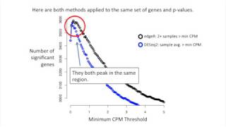
StatQuest: edgeR and DESeq2, part 2 - Independent Filtering
StatQuest with Josh Starmer
The Main Ideas of Fitting a Line to Data (The Main Ideas of Least Squares and Linear Regression.)
StatQuest with Josh Starmer
The Sum of Regrets
StatQuest with Josh Starmer
Lowess and Loess, Clearly Explained!!!
StatQuest with Josh Starmer
StatQuest: Hierarchical Clustering
StatQuest with Josh Starmer
StatQuest: K-nearest neighbors, Clearly Explained
StatQuest with Josh Starmer
Your Dark Side
StatQuest with Josh Starmer
Boxplots are Awesome!!!
StatQuest with Josh Starmer
What is a (mathematical) model?
StatQuest with Josh Starmer
Linear Regression, Clearly Explained!!!
StatQuest with Josh Starmer
Linear Regression in R, Step-by-Step
StatQuest with Josh Starmer
Maximum Likelihood, clearly explained!!!
StatQuest with Josh Starmer
Brothers
StatQuest with Josh Starmer
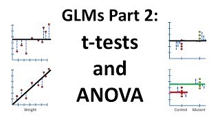
Using Linear Models for t-tests and ANOVA, Clearly Explained!!!
StatQuest with Josh Starmer
StatQuest: How to make a Mean Pizza Crust!!!
StatQuest with Josh Starmer
StatQuest: A gentle introduction to RNA-seq
StatQuest with Josh Starmer
I'm Alive
StatQuest with Josh Starmer
StatQuest: t-SNE, Clearly Explained
StatQuest with Josh Starmer
More on: ML Maths Basics
View skill →


Related AI Lessons
⚡
⚡
⚡
⚡
I Spent Weeks Looking for a Research Gap Before I Realized I Was Searching the Wrong Way
Medium · AI
ICMI 2026 Reviews [D]
Reddit r/MachineLearning
Workshop submission for main conference paper under review [D]
Reddit r/MachineLearning
Kept context-switching between arxiv, OpenReview, GitHub, and HuggingFace for every paper, so I built this. Chrome extension + website with everything inline, plus citation graph + SPECTER2 neighbors. 3M papers, free, feedback welcome [P]
Reddit r/MachineLearning
Chapters (9)
Awesome song and introduction
1:19
Overview of what t-SNE does
2:24
Overview of how t-SNE works
4:12
Step 1: Determine high-dimensional similarities
9:26
Step 2: Determine low-dimensional similarities
10:33
Step 3: Move points in low-d
11:05
Why the t-distribution is used instead of the normal distribution
6:17
I should have said that the blue points have twice the density of the purple poi
7:08
There should be a 0.05 in the denominator, not a 0.5.
🎓
Tutor Explanation