Time Series Talk : Seasonal ARIMA Model
Key Takeaways
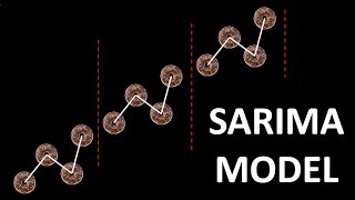
The video introduces the Seasonal ARIMA model for time series forecasting, incorporating seasonality into the model and explaining its 7 parameters. It also covers the ARIMA model with seasonal components, using the back shift operator, and defining a new variable to make the time series more stationary.
Full Transcript
this video we're finally gonna start talking about how to incorporate seasonality into our Rhema model so there's gonna be a lot of moving parts throughout the video so I want to go really really slowly and kind of form a foundation for why we're doing this talk about some notation talk about one of the simplest models and then we're gonna go even even simpler and talk about just what happens when we reduce this to its bare bones okay so first things first the ARIMA model if you remember from a previous video was the autoregressive which is saying that i want to predict the value of my time series today based on the value of the time series some periods in the past integrated which means my time series has some sort of upwards or downwards trend so I'm using different synced in order to get rid of that to make it stationary moving average which means that I'm using my air from a previous period to inform my prediction of my time series today and the new thing we see here is this s so that s stands for seasonality which means that on top of the whole ARIMA model we also have seasonality which if you remember from the seasonality video what that means is a repeating pattern within a year that happens over and over and over again over time so that's all the pieces of it let's see how they factor into this chart here here's the setup for this model you are a doughnut salesman and every every three months you record the number of doughnuts that you sold up until then and you record them on this graph here so this is my donut drawing this is why I was a math major not an art major because that does not look like a donut but we're gonna continue here we see that we start in 2014 15 16 17 18 and 19 and there's four dots inside of every year which means that every three months right because 3 times 4 would be 12 total months you're recording the number of donuts sold and we see a very very clear seasonal pattern we see this W type thing repeating every single year so check box on the fact that there is seasonality in here okay so how do we know that we should use a surry mo model here so seasonal ARIMA sometimes sarima model we know that their seasonality so that's a check you actually take a color here and put check check we know their seasonality we know that there might be a RMA component because the value of something at some period depends on the value of it maybe for periods ago it seems like so ma and AR are possible checks what about the integrated we see there's a clear upward trend over time that we're going to need to account for if we're going to correctly predict this so all of these pieces are checks or potential checks so we're clear to start thinking about using this ARIMA model here now the first thing I'm going to do is show you some notation and it looks a little bit scary at first but we're gonna go from complicated to simple so we're gonna show you the notation say what it all stands for and then we're gonna fill in some concrete numbers and talk about what happens to the model in all of those cases okay so a serving of model or a seasonal or rima model is given by seven whole parameters three of these you're already familiar with the P the D and the Q so the P corresponds to the order of the AR piece the D to the order of the integrated piece or how many times we take a difference to get it to be stationary and the Q to the order of the MA piece now the good thing about these seven parameters is that these next three are kind of just analogues of the first three except in a seasonal context so actually before talking about the uppercase P upper case D uppercase Q it makes more sense to talk about lowercase M lowercase M is the seasonal factor which is the number of periods within a year it takes for the seasonality to repeat in our case that's four because we see that within a year so 2014-2015 for example we see one two three four periods and then after that from 2015 to 16 again these four periods form the next batch of seasonality so basically if you were to batch up your seasonality this is the number of terms within a year that your seasonality you get that seasonality at so M is four for us in this case now going back to this uppercase P uppercase D uppercase Q these are the analogs of the lowercase versions of these except for the seasonal components so for example I'm gonna plug in some real numbers here and they're all going to be one in this case except for the M which is for of course what this model is saying okay ARIMA 1 1 1 and then uppercase letters being 1 1 1 as well this is saying that I want to integrate my model or take the first difference of my model which is that D red here and that corresponds to I'm using the back shift operator the B operator same thing as L if you remember our lag operator video so that one corresponds to this piece right here which is saying back shift my whole time series I'm apologize that corresponds to this piece here that says back shift my whole time series by one period so Y sub 2 - y sub T - 1 now this one the capital D says back shift my entire time series also by four time periods why four because that's M so M applies to this upper case P D and Q and in the same way that P the lower case P D and Q there's like a secret one here you can think about it that way because we're only doing that for one period okay so next this AR piece right here this AR one corresponds to what I was pointing at earlier actually which is I want to take into account the time period the time series one period ago into my prediction this one which is the upper case P which is the order of the seasonal AR bit is going to be given by this guy right here which says I have a different coefficient upper case fee which is this guy right here and I want to back shift my time series four periods in the past because that's my M you can probably see where I'm going with this this is the MA piece for the standard component which is given by that guy right here and the final one is the MA piece for the seasonal component which is given by this right here the only difference is the difference parameter which is upper case theta sub one and I want a back shifted four periods in the past by it I mean the error okay that was very very confusing so we are going to go even simpler and set a bunch of stuff to zero so that we can actually expand one of these models because if you think about expanding this entire mess you're gonna get so many terms that it's gonna be disgusting so we're not going to be expanding that entire model we're gonna be setting a bunch of stuff to zero here's a very very simple case we're gonna do lookit ARIMA we're lowercase P is 1 and then these other guys are 0 uppercase D and uppercase Q are both 1 M is 4 and this guy is 0 here okay so this is a little bit more manageable and it's gonna actually be more instructive in what we're actually doing behind the scenes because right now it's not very clear okay so we're doing here as we're saying I want to predict my time series y sub T based on the time series 1 period ago that's what this is saying right here and that's what's encoded by this back shift operator with a 1 exponent if you want to think about it that way I also want to take the difference from four periods ago that's what this uppercase D being one says and that is encoded by this one - back shift four periods ago on my time series the last thing I want to do is take a moving average a seasonal moving average from four periods ago that's what this guy is doing here okay taking the moving average four periods ago for the error now this is a little bit easier to expand I'm going to expand these two polynomials basically multiply them together so I get 1 minus C sub 1 B minus B to the power of 4 plus because negative negative makes a positive fee sub 1 B to the power of 5 because this is B one before combined they become B 5 apply to Y sub T is equal to this error multiplied by the 1 is just itself plus uppercase theta sub 1 this error back shifted for periods in past is epsilon sub T minus 4 all right we're almost there now I'm going to take this Y sub T and hit it against all of these terms here so we get Y sub T we get minus so actually I did a little bit of refactoring here as well because I did this B to the power 4 and that state here I took all the other terms on this side of equal sign which is why you're seeing fee sub 1 Y sub t minus 1 minus V sub 1 Y sub T minus 5 Plus these terms we already had now you're probably thinking I just made a huge mess but it's about to get real clean if we define a new variable called Z sub T which is defined as Y sub T minus y sub T minus 4 going back to the graph for a moment this is saying I have a new time series which is defined as the original time series at some point - that time series for periods ago which makes sense because that's going to help me get this time series from an upward trend to more stationery if I do that then this of course by definition is Z sub T I can factor out the fee sub 1 and I'm left with Y sub t minus 1 minus y sub T minus 5 which again using this identity is just Z sub t minus 1 and these guys stay how they are now this makes a lot more sense and let's talk through that to end this video this is saying that I want to make a prediction about my new time series Z sub T which again is the difference diversion of my original time series to do that I'm going to be saying that it's gonna be some parameter V sub 1 times that new time series 1 period in the past plus some other parameter times my error for periods in the past plus my error today so we can see all the pieces at play here and there was three pieces right the first piece was this integrated bit the seasonal integrated bit of order 1 but of course that's for periods ago how is that taken into account that's taken into account by the fact that Z sub T is that difference from the current period to four periods ago how do we factor in the AR one component which is not seasonal of course that's right here because this is t minus one and this is just t and lastly how do we factor in the seasonal moving average component that was has the seasonal factor of four on it of course that's taken care of by the fact that we're also predicting based on the error for periods ago okay so hopefully even though it's confusing at these stages once you simplify it you see where all of these factors eventually appear and you can generalize by substituting other things as not zero or setting certain things equal to zero okay so please if you have any questions I encourage you to put them in the comments I know that the more letters get added to this big acronym the more confusing it gets but I was hoping that this is a good first introduction into the sarima model in time series analysis okay so until next time
Original Description
Intro to the Seasonal ARIMA model in time series analysis.
Playlist
Uploads from ritvikmath · ritvikmath · 55 of 60
1
 2
2
 3
3
 4
4
 5
5
 6
6
 7
7
 8
8
 9
9
 10
10
 11
11
 12
12
 13
13
 14
14
 15
15
 16
16
 17
17
 18
18
 19
19
 20
20
 21
21
 22
22
 23
23
 24
24
 25
25
 26
26
 27
27
 28
28
 29
29
 30
30
 31
31
 32
32
 33
33
 34
34
 35
35
 36
36
 37
37
 38
38
 39
39
 40
40
 41
41
 42
42
 43
43
 44
44
 45
45
 46
46
 47
47
 48
48
 49
49
 50
50
 51
51
 52
52
 53
53
 54
54
 ▶
▶
 56
56
 57
57
 58
58
 59
59
 60
60

Math Team Update
ritvikmath
Single Variable Calculus Volume of a Sphere - Proof 1
ritvikmath
Single Variable Calculus Volume of a Sphere - Proof 2
ritvikmath
Multivariable Calculus Volume of a Sphere Proof - Triple Integrals
ritvikmath
Multivariable Calculus Volume of a Sphere Proof - Double Integrals
ritvikmath
The Euclidian Algorithm
ritvikmath
Proving the Chain Rule
ritvikmath
Proving the Fundamental Theorem of Calculus Part 1
ritvikmath
Proving the Fundamental Theorem of Calculus Part 2
ritvikmath
Math Puzzle - Poison Perplexity
ritvikmath
Math Puzzle - Poison Perplexity - Solution
ritvikmath
Expected Value and Variance of Continuous Random Variables (Calculus)
ritvikmath
Expected Value and Variance of Discrete Random Variables (No Calculus)
ritvikmath
Array Method
ritvikmath
Complex Power Series and their Derivatives
ritvikmath
Distributions - Intro
ritvikmath
The Poisson Distribution
ritvikmath
The Bernoulli Distribution
ritvikmath
The Binomial Distribution
ritvikmath
The Continuous Uniform Distribution
ritvikmath
The Geometric Distribution
ritvikmath
The Triangular Distribution
ritvikmath
The Exponential Distribution
ritvikmath
The Borel Distribution + Notes on Poisson Distribution
ritvikmath
The Gamma Distribution
ritvikmath
The Normal Distribution
ritvikmath
The Laplace Distribution
ritvikmath
The Chi - Squared Distribution
ritvikmath
Overfitting
ritvikmath
Vector Norms
ritvikmath
Truths Behind the Titanic : K-Nearest Neighbor
ritvikmath
The Mathematics of Breakups
ritvikmath
Sillyfish
ritvikmath
Finding Optimal Paths - Dynamic Programming
ritvikmath
HowToDataScience : Scraping Twitter Data
ritvikmath
Decision Trees
ritvikmath
Perceptron
ritvikmath
Naive Bayes
ritvikmath
K-Nearest Neighbor
ritvikmath
Evaluating Machine Learning Models
ritvikmath
Decision Tree Pruning
ritvikmath
K-Means Clustering
ritvikmath
Gaussian Mixture Model
ritvikmath
Data Science - Fuzzy Record Matching
ritvikmath
Time Series Talk : Autocorrelation and Partial Autocorrelation
ritvikmath
Time Series Talk : Autoregressive Model
ritvikmath
Time Series Talk : Moving Average Model
ritvikmath
Time Series Talk : ARMA Model
ritvikmath
Time Series Talk : ARCH Model
ritvikmath
Time Series Talk : White Noise
ritvikmath
Time Series Talk : Stationarity
ritvikmath
Time Series Talk : ARIMA Model
ritvikmath
Time Series Talk : Lag Operator
ritvikmath
Time Series Talk : What is Seasonality ?
ritvikmath
Time Series Talk : Seasonal ARIMA Model
ritvikmath
So ... What Actually is a Matrix ? : Data Science Basics
ritvikmath
Derivative of a Matrix : Data Science Basics
ritvikmath
Basics of PCA (Principal Component Analysis) : Data Science Concepts
ritvikmath
Eigenvalues & Eigenvectors : Data Science Basics
ritvikmath
The Covariance Matrix : Data Science Basics
ritvikmath
More on: ML Maths Basics
View skill →

![AI With Python Full Course 2026 [FREE] | Learn Artificial Intelligence With Python | Simplilearn](https://img.youtube.com/vi/IvFW-r_S6UI/mqdefault.jpg)



Related Reads
🎓
Tutor Explanation

 DeepCamp AI