The Normal Distribution

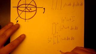
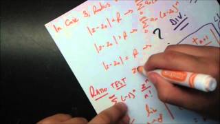
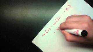
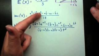
In this video, we'll be talking about probably the most famous distribution that most people learn about at a very usually early age. They kind of get a notion of it, the normal distribution. So, this is kind of what people think of when they say the bell curve. Uh the one that usually looks like this uh and is used for many different applications and uh things like that. So, it's usually more symmetric than that. But, uh okay. So, we say that a random variable X is distributed as normal with two parameters mu and sigma squared. So, since this is sigma squared, this has to be positive. Mu on the other hand can be any real number. Okay, so I'll maybe make a quick note of that sigma squar must be greater than or equal to zero and mu can be any real number. So we say that if it has the following PDF and this is probably the most complicated PDF, most complicated PDF that we've seen so far, but um it'll quickly become very familiar because this is used so often. So we write our familiar PDF form f big X and we have little X is equal to and the thing about this PDF is that it has no other conditions. Usually we have a case where it's zero otherwise. Here it's just one thing and it's applies to the whole real line. So it's 1 / sigma<unk> 2 pi uh e to the x - mu^ 2 all over 2 sigma^ 2. Okay. So it is 1 / this sigma * radical 2 pi e to the whole thing up here. Okay. So uh it's not too complicated but uh it is more complicated than other things we've seen so far. And there's not really uh we're not really going to give it an intuitive way to think about it here. So maybe that might make it harder to memorize, but try to memorize it best as possible. Okay, cool. So this is it. This is on the whole real line. X can be anything from minus infinity to infinity. And indeed, if you integrate this from negative infinity to infinity, you will get one. Okay. Um so the next thing we're just going to go dive right into how to find the expected value. Uh the variance I've done on the back of this paper. We'll just trace through it and then we'll do the moment generating function uh as well. Okay, so let's do the expected value first. So, uh, let me use a different color maybe. So, we want to find the expected value. So, we're just going to do the standard thing. Expected value of x is given by the integral negative infinity to infinity. And here we don't change the bounds because it is indeed from negative infinity to infinity. We'll write the uh PDF. So, write the PDF. Uh, and then since we're doing the expected value, I want to put an extra x in here. dx. Okay, this looks very complicated and uh there's a few tricks we're going to have to learn along the way. So, let's do the simplification we can. This right here is a constant. This sigma radical 2 pi is a constant. We're going to pull it right out. 1 / sigma rad 2 pi integral from minus infinity to infinity. E - x - mu^ 2 over 2 sigma^ 2 and we have an x out here dx. Now, the next thing I want to do is make a substitution. I'm going to do a u substitution and I'm going to go ahead and use the choice uh u = x - mu over sigma because that is kind of what's here except it's squared. So then if I have that I have du = 1 / sigma dx. Okay. Uh so now I'm ready to make my u substitution. So I have 1 / sigma radical 2 pi. Uh do the bounds change at all? If I put negative infinity into here for x, this is still negative infinity. If I put uh infinity, it's still infinity. Notice sigma is the positive square root of the sigma squar. Okay, so it's positive. So I'm still getting from minus infinity to infinity. Uh this x becomes what? It becomes u sigma + mu. U sigma + mu. Uh and then I get e to the u ^2 / 2. Uh okay. So that makes sense because this is if you square this it becomes this except you still have to put it / 2. And this dx changes to what? This dx changes to a sigma du. So it changes to a du. and I'll put the sigma outside since it's a constant and it nicely cancels with the bottom sigma right there. So we have 1 over radical 2 pi as a constant that's outside. Okay, now we're going to split this as two integrals because there's a plus sign here. So we're going to get on the one hand we're going to get 1 / radical 2 pi that's just going to be on the very outside. The first integral is going to be uh sigma integral from minus infinity to infinity of u eus u ^2 / 2 du which is going to be we can use regular means to calculate this guy and on the other hand it's going to be plus mu integral minus infinity to infinity e^2 / 2 du. Okay cool. So this guy is going to be what we could go ahead and do our calculations but let's notice something. This inside this integrant is an odd function because this u ^2 over two is an even function and this makes it odd. Which means that if we integrate an odd function from a negative uh limit to the positive limit and the negative and positive absolute values are the same. In this case they're negative infinity and positive infinity this whole integral will just go to zero. Okay. So that simplifies things a lot very nicely for us. So really all we have is mu over rad 2 pi. Uh this integral this integral it's not clear how to do it at first. So, we're going to have to do a little bit of creativity. We're going to have to use polar coordinates here. So, instead of calculating this integral, let's calculate this integral squared. I know that seems weird. Why would you complicate it? But we're going to see why that makes sense. So, we want to calculate I'm going to take I'm going to try to calculate this integral squared. So, I want that integral times itself. So, I'm going to write exactly that. So, uh I'm going to write again a copy of that except I'm going to use a different variable. And it really doesn't matter which variable I use here because if I calculate this integral and this integral, they'll be the same because this might be in respect to u. This might be with respect to s, but in the end they're going to have the same answer. So I'm really getting this integral squared still. Now since uh these this ds and this du are independent. They have nothing to do with each other. I can kind of merge these guys together in the following sense. I can have a double integral minus infinity to infinity minus infinity to infinity uh e to the and since I'm going to multiply these integrants together I can add their exponents so I have e to the minus uh u ^2 + s^2 all that over 2. Okay. And then I have du ds. So you're probably thinking why did I do this? This seems like a very just messing things up. But now we're ready to make that polar change of variables. And that change of variables uh the polar change of variables will be r^2= u ^2 + s^2. Uh so we're going to try to change this into something in the form dr r d theta. So changing into polar uh go back and review that if you need to. But um since it's on the whole plane negative infinity to infinity in the x and y or in this case the u and s uh it's going to be we're going to let the outside integral be theta. So we're going over the whole circle and the whole this r will go from 0 to infinity. The radius is going to be from 0 to infinity and we're going over the whole circle in the polar form. Now e this inside becomes very nice which is why we're doing this becomes e r 2 / 2 and this d remember when you change this part it becomes rdr d theta. So we put r and then we put uh dr r d theta. Okay so I run out of room so let me grab another piece of paper. Okay, this will work nicely. So what we have here is this. And all we need to do now is just simplify this a little bit further. Uh so we're going to have uh this inside part is the same kind of integral we would have evaluated up here if we wanted to evaluate it. Now we have to evaluate it. So we're going to u substitution. U let me use z instead because we've used u for something else. So we have z = r 2 / 2. Okay. Uh so dz = rdr. So inside we're going to have uh does does the integrants change at all? So zero stays zero. Infinity stays infinity. So sorry do the limits change at all? No they don't. Um this rdr becomes a dz and here we have e to the minus z. Okay so this is easy to evaluate. This is just e to the minus z evaluated from 0 to infinity. So it's e to the when you put eus infinity you get 0 - 1. So this just comes out nicely as 1. So really this whole inside part right here is just one. So really we have the integral 0 to 2 pi uh 1 d theta. So it's just equal to 2 pi. Now so we found that this integral this one right here squared was 2 pi. So by itself it's just radical 2 pi. So this is radical 2 pi. And notice we have a negative we have a radical 2 pi on the denominator to cancel that. So this cancels with this. And all that survives after all of this kind of mess is mu. And that's pretty clean. So we find that a normal distribution with parameters mu and sigma squar if you want the mean all you have to do is look at that first parameter the mean is given by mu which is kind of suggestive because mu mean you know kind of a it's very suggestive in its name so that was very easily done now the variance uh it's a similar calculation I've done it for you let's walk through it variance remember is expected value of x^2 minus expected value of x squar we just found that was mu so mu^2 down here now we need to calculate this expected value of x^2 so I did the same exact thing. You know, I found the I took the PDF. I multiply by X^ squ here and I've taken the constants out. I immediately made that U substitution again. X - mu over sigma and it became a little bit more complicated cuz I had to square it here. So, I have split up into three integrals. This one, this one, and this one. Turns out this one is the same form that goes to zero. So, that went to zero for us. Uh let's see. This one right here, we just calculated that this was uh rad 2 pi, which is why that showed up here. And this was kind of a new integral. uh we didn't really know how to do it yet, but it turned out a simple integration by parts worked out. If we let v= u and dw= u e u ^2 over 2du. So that integration by parts is carried out. We see that this becomes radical 2 pi as well. So really we have 1 / radical 2 pi sigma rad 2 pi plus mu^2 rad 2 pi becomes very nice sigma 2 + mu^2 subtract the mu^2 we need to subtract and you get sigma squar is the variance. So again look at the parameters to find the variance. All you have to do is just look at this uh parameter right here. So that's the way normal distribution is defined. It's defined in terms of its mean and its standard deviation. So in a in a graph for example let's give concrete values. Let's say mu is -1. Let's say sigma is maybe one. Okay. So that means it's centered at negative 1. That means this bump which you usually think is at zero. In this case it will be at ne1. So here's the actual zero. Here's one maybe here's minus one. So that that hump will be centered up here. And the bigger the standard deviation is, the more kind of spread it'll be. That's kind of a colloquial measure. It's called the spread. So uh maybe we'll just draw a quick picture here. So it's going to look a little bit like that maybe. Okay. So the point is here it's centered at one. So maybe for reference, if I had changed the sigma square to two instead, it would be spread out more. So maybe uh let me do this in different color. Let me attempt to do this. So if we put the mean, notice, would still be at ne1. So that hump would still be at negative one, but now it's kind of spread out more. Kind of like that, right? So it's spread out more. Um that's the basics of it. So uh now we can kind of go in and compute the moment generating function. So let me let's continue on this piece of paper right here where we have that. So we're trying to find the moment generating function of this normal random variable. So we could go through that whole process and make this hard on ourselves or we could use the property of the moment generating function and then we could just do it for the standard normal random variable. So the standard normal random variable is the normal with mean zero and variance one. And it turns out this has very nice properties and it makes calculations a lot simpler for us. So we're going to work with this guy. The PDF of this guy is given by if we plug mu= 0 and sigma^2 is 1. It's just 1 / rad 2 pi e x^2 / 2. Okay, that it looks a lot nicer than the general form. Now what we want to do is find the moment generating function of this guy. How do we do that? Remember it's expected value e to the sx. So doing that it's going to be minus infinity to infinity. Uh let's take the one over 2 pi out. Um we need to put e to the sx e x^2 / 2 dx. So all we have to do is some um creative factoring here and then it kind of solves itself. So we went over add 2 pi. Let's first just combine the exponents. We have e to the sx - x^2 / 2. uh we have dx. I'm going to rewrite it in the actual form and then we'll just confirm that it's correct. So we have 1 / radical 2 pi uh and I forgot my bounds here. So minus infinity to infinity and we're going to have e to the power of -2 x - s^2 + 12 s^2. Let's make sure this is correct. So if we expand this, let's do the expansion maybe up in this corner right here. So if we have -2 x - s^2 that expands to -2 x^2 - 2x s + s^2 and then we have that + 12 s^2 + 1/2 s^2. So we see right off the bat this - 1/2 s2 squ this plus 12 x s2 cancel. So all we're left with is just this -2 x^2 uh plus xs and that we see is exactly what we have here. We have this sx uh -2 x^2. Okay. So this is correct and it makes it nicer for us because now we can take this e to the 1/2 s^2. It has nothing to do with um x. So we can just take it out. So we have 1 / rad 2 pi uh we get e to the 12 s^2 integral infinity to infinity uh e to the -2 x - s^2 dx. Now let's notice something. So I'm going to actually take this 1 over 2 pi and put it with this just so we can notice this fact. But we have e to the s^2 / 2 still sitting outside minus infinity to infinity 1 / radical 2 pi uh e to the - s - x^2 x - s^2 over 2 dx. Now notice this is the pdf of a normal I'm just going to shorten normal to n for here. normal uh s and variance one random variable, right? Because u the normal this mean s shows up up here and the variance is one because sigma squar being 1, it would show up down here as 1 squ and would show up here as 1. So this is exactly that. And so we're taking it over the whole real line. Since it's a probability density function, it must integrate to one. So this whole integral must be one. A very easy way to evaluate this integral. So really all we're left with is just this outside term is e to the s^2 / 2. So, we've successfully found the MGF of a normal uh 01 random variable. But that's not fully what we wanted. We wanted to find the MGF of a general uh you know normal random variable. And I've written a almost full write up here. We're going to complete the last few steps together. So, we want to find the mgf of a normal mu sigma squared. So, the steps are not that hard. The real insight is the thing we just did. So, at the beginning, I just started by saying I wrote exactly what it is. It's 1 / sigma rad 2 pi. That's part of the PDF. Uh negative infinity to infinity e to the sx. That's the mgf coming in and we have the rest of the PDF here. So I used the regular u substitution we've been using u= x - mu over sigma and I carried that through. So you can look through the algebra if you want and I've gotten to this step here. Now this is what if we looked back at what we had uh when we were finding the mgf of a normal 01 random variable we had this. We had 1 / radical 2 pi negative infinity to infinity e to the sx e^2 dx. Now compare that with what we have right here. Okay, here we have that exactly 1 over rad 2 pi e to the now the only change here is that this is a s sigma instead of just an s. But notice s was just a real number. Sigma is just a real number. So what we're going to take the final answer and everywhere we see a s we're going to replace it with a s sigma. Okay. So since the final answer was e to the s^2 over 2. Here the final answer is e to the s sigma^ 2 / 2. Multiply that by what's on the outside here and we get uh e to the mu s e to the s^2 sigma^ 2 all over two and that is the mgf of some general normal mu sigma squ uh random variable distribution. Okay, so that is uh that's that's that's mostly what we're going to say about the normal distribution in this video. Uh we're going to have a lot more to say about it because the normal distribution and the kai square distribution uh have a relationship.