Explainable AI explained! | #5 Counterfactual explanations and adversarial attacks
Skills:
Research Methods90%Reading ML Papers80%Paper Reproduction70%AI Alignment Basics60%ML Maths Basics50%
Key Takeaways
The video explains counterfactual explanations and adversarial attacks in the context of Explainable AI, covering concepts such as counterfactual explanations, adversarial attacks, and black box models, and demonstrating tools like Dice library and TensorFlow.
Full Transcript
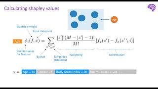
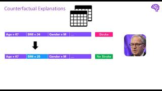
[Music] hi everyone welcome back to this explainable ai series in the last videos we've seen different interpretability techniques to better understand black box machine learning models these methods mainly produced feature importances and showed us how the inputs affect our prediction today i want to talk about another type of explanation which is usually called a counterfactual in my opinion it's a pretty powerful approach and i hope that at the end of this video you will be familiar with it as well let's start with an intuitive basic explanation of what counterfactuals are in the second video i introduced the data set for this series which is a binary classification problem for stroke prediction we said that our test patient john is interested in why he gets a certain prediction from our model previously our explanations using sharp and lime had a form like h is the most important feature or the higher h gets the higher the stroke risk will be and so on so these were mainly feature importances and dependency plots now counterfactuals go in another direction here we want to tell john what he could do to avoid a stroke so it's a counter fact that gives him the possibility to change the situation a counterfactual could look like this hey john right now your prediction is 90 stroke if you would decrease your body mass index to 25 the prediction would be 70 no stroke so the orange part here is now the counterfactual which is just another data point that leads to a different prediction we can think of it like a newly created person that would end up with no stroke so all values for our data point for john stay the same just body mass index is changed to another value and if this is done we get another output for our black box model which is highlighted in green we can also give a more formal prediction for counterfactuals generally a counterfactual is the smallest change in the input features that changes the prediction to another output just like in our example going from stroke to no stroke just a side note counterfactual explanations are sometimes also called contrastive explanations in the literature so here i wanted to visualize the basic idea for tabular data one instance so one row in the tabular data set corresponds to one person and the columns are the different features our model uses so age body mass index and so on so all we have to do now is change a specific value of our inputs so that the prediction alters to the target class for example no stroke it was shown that providing explanations of that sort so counterfactuals lead to a high explanatory value for humans counterfactuals exist already a long time in psychology a theoretical definition was initially presented by lewis in 1973. the idea for using them in machine learning was first presented in a paper called counterfactual explanations without opening the black box this paper was published in 2017 the basic idea for calculating counterfactuals comes from a different ai field which is also called ai safety the goal in this field is to make machine learning models more secure against manipulation adversarial examples are well-designed input samples that use the shortages of machine learning algorithms to generate false predictions an example for this is this classifier for which the input on the left is slightly changed by adding adversarial noise in the middle as a result the prediction changes from panda to gibbon the approach to generate adversary examples is quite similar to generating counterfactuals as both look for the minimal changes in the input to generate a different output in both cases we want to solve the following optimization problem find x prime which is the counterfactual or adversarial sample that changes the prediction of our black box model to a target class c in the example on the left access the panda image with a panda prediction and on the right we would have x prime which is the adjusted input that leads to a given prediction in this optimization problem on the right we also see a distance function d which is minimized this distance function makes sure that we stay as close as possible to the original inputs that's because we still want to have a panda on the image but aim to get a different prediction by our blackbox model so to summarize it in both cases when explaining black boxes and also when attacking black boxes we want to find a similar input data point that changes the prediction if you are further interested in the second case adversarial attacks i've also uploaded a video on how to code that for convolutional neural networks okay so now we know what counter factors are and how they can be formulated mathematically but how do we calculate them in real life there exist several approaches to compute contractuals for a prediction all we need to do is solve the previously presented optimization problem generally the approaches can be divided into white box and black box approaches if we have access to the model internals such as the weights in the neural network then that is perfect and we can use this information to faster find the minimum in the optimization problem for example in a neural network we can simply calculate gradients for our problem that guide us using gradient descent if we don't have access we need to rely on the relationship between inputs and outputs that means we have to find a solution by querying the model many times that is the model agnostic way of calculating counterfactuals while the white box approaches on the left are model specific for both categories many different ideas exist and i won't go into the detail of the individual papers however here i linked some references if you want to read more about this topic just an example the work for certif ai uses a genetic algorithm to create counterfactuals that means it uses selection mutation and crossovers so the typical operations in evolutionary algorithms the work by vachta et al is model specific and uses an atom optimizer and gradient descent to find the optimal counterfactual all of these approaches perform some sort of perturbation on the input that means they change the feature values either randomly or guided in some way to better explain this let's again quickly jump to our tabular example here we would for instance randomly change values such as here we decrease the body mass index to 32 we do this many times for example again for 29 and then again for 22. the last change would flip the prediction to no stroke if we do this many times we get a good approximation of the decision boundary for our model and can determine the minimal changes that are required to predict no stroke and then we can use this information and tell to this person for example john hey if you decrease your body mass index to 22 you will probably not get a stroke again this approach is model agnostic and quite similar to brute force but if we can use the model internals we can apply these feature changes more intelligently this approximation of the decision boundary is also nicely visualized by this example from dice which is a counterfactuals python library by microsoft in this example they want to provide an explanation why a loan has been approved or rejected and how to change the situation at this point you might say wait a minute there are many different possibilities for counterfactuals in this example we can either increase the income by ten thousand dollars or we increase the income by five thousand and have one more year of credit history both will get us on the other side so both will get the loan approved so what is the best counterfactual well there is no best both are valid counterfactuals and we cannot really say which one is better this behavior is also known as the rashomon effect that's why this python library i just talked about produces several counterfactuals so for example five dice so the name of the library stands for diverse counterfactual explanations that simply means we want several counterfactuals that are as different as possible this gives us the option to select the most suitable explanation for our personal situation so now that we are familiar with all the concepts let's switch to the code and compute some counterfactuals so here we are in vs code again and just like in the other videos we imported the data the random first model which is our black box classifier and some metrics to calculate the performance of our model so let's run this and you've seen this many times now import the data and we have one second we have a shape of that for the test and train data and then we fit the model which again is having a nice accuracy but imbalanced data sets so our f1 score is not so nice all right and now we come to the contractual part so this is the library i previously talked about you can install it running pip install diceml and it will create several so diverse contractual explanations for us for this library we need to create two things we need a data object and a model object the data object tells us what the data input looks like if there are continuous features that's important because if we want to perturbate the features for example increase or decrease age we need to consider discrete features and continuous features because they have different perturbation strategies so we need to manually pass in which features are continuous in our data set and then we also specify here what is our target variable and then here in the data frame section we pass in the data from our data loader okay in the model part we simply pass the model and we select the back ends so there are back ends for tensorflow pytorch and many others and i will select cycle learn as this model comes from scikit-learn so now using those two things so the data which is called data dice here and the random forest dies which is the model object we can create this explainer instance which is called dice and here we can specify which methods we want to use for generating counterfactuals as i said there exist model agnostic in model specific approaches the most model agnostic one is random sampling but also genetic algorithms and other optimizers are available if you have a deep learning model you can of course use an optimizer for deep learning that simply uses the gradients so here's an overview this is the github page from dice and here are some of the methods so they call it gradient based so that's model specific methods specifically designed for neural networks and for model agnostic approaches they have those three okay that's pretty much it regarding what we need and now what we can do is let me just quickly run this now we can select input data points so as i said this approach is a local explanability approach so we need to select a single data input we can use for our generation and then we call this function generate counterfactuals on the explainer object we created over here and we pass our input data point which is simply a first sample in my test data set and here i specify i want three counterfactuals so three diverse counterfactuals to be generated and as this is a binary classification problem so the stroke prediction data set i can simply pass in here opposite so it will flip the class so let's run this and the second function down here is then so this generates us the counterfactual and then i can call on this counterfactual objects a function called visualize as data frame and this will show us what is the input so what is this individual data sample and what are the three counterfactuals that were generated okay so first let's have a look at this query instance so we see that the original classification was zero so no stroke for this first data point and this is based on our random forest model and we see this is a male uh merits and all the other features and we can see 70 years old body mass index of 30.4 and a glucose level of 72. and now when i call this visualize as data frame i can pass in show only changes that means this table down here will only show the differences to this data points so as i said a counterfactual is just another data point that is slightly changed from this individual input and we can see we see some values that changed in the middle here which is work type private but especially we have many changes regarding body mass index so apparently if the body mass index is too low the stroke risk increases again i wouldn't trust this model but this is just for this example so here we have three counterfactuals that suggest us to decrease the body mass index to get a stroke prediction so usually we would go in the other direction and say when do you not get a stroke prediction but in this example we just select stroke because this first data point is no stroke okay so of course body mass index 0.9 doesn't really make sense that's why we also have the option to pass in feasibility criteria for example you can say only change those features because usually you cannot change from male to female for example and additionally we can also say the permitted ranges for changes must lie between those two values and there are in this library a couple of additional options to ensure that we get feasible counterfactuals so counterfactuals that actually make sense so if i run this again i can pass in those two parameters into this generate counterfactuals function again again we want to generate three counterfactuals for the opposite class but now using this feasibility criteria so again we get the same outputs but now we should see okay here we have changes that lie within the permitted range so now it says you need to change the body mass index to the specific value and no other changes in this example so if you would have a more complex models you would have changes at several positions but again a counterfactual is the minimal change to change the prediction and here apparently the minimal change is to decrease the body mass index by around 10 and again we also don't have a lot of diversity in this model that's why those three diverse counterfactuals are still quite similar that's just because the model is not so good alright that's it about counterfactual explanations today i hope you find them as powerful as i do and if you have further questions just let me know in the comments the code is again available on github the link is in the description the next video will be the last part of this explainable ai series where we have a look at layer-wise relevance propagation a method which is specifically designed for neural networks
Original Description
▬▬ Resources ▬▬▬▬▬▬▬▬▬▬▬▬
Github Project: https://github.com/deepfindr/xai-series
CNN Adversarial Attacks Video: https://www.youtube.com/watch?v=PCIGOK7WqEg&t=1140s
▬▬ Timestamps ▬▬▬▬▬▬▬▬▬▬▬
00:00 Introduction
02:58 CFs and Adversarial Attacks
05:15 Generating CFs
07:55 Rashomon effect
09:20 Code
▬▬ Support me if you like 🌟
►Link to this channel: https://bit.ly/3zEqL1W
►Support me on Patreon: https://bit.ly/2Wed242
►Buy me a coffee on Ko-Fi: https://bit.ly/3kJYEdl
Watch on YouTube ↗
(saves to browser)
Sign in to unlock AI tutor explanation · ⚡30
Playlist
Uploads from DeepFindr · DeepFindr · 13 of 56
1
 2
2
 3
3
 4
4
 5
5
 6
6
 7
7
 8
8
 9
9
 10
10
 11
11
 12
12
 ▶
▶
 14
14
 15
15
 16
16
 17
17
 18
18
 19
19
 20
20
 21
21
 22
22
 23
23
 24
24
 25
25
 26
26
 27
27
 28
28
 29
29
 30
30
 31
31
 32
32
 33
33
 34
34
 35
35
 36
36
 37
37
 38
38
 39
39
 40
40
 41
41
 42
42
 43
43
 44
44
 45
45
 46
46
 47
47
 48
48
 49
49
 50
50
 51
51
 52
52
 53
53
 54
54
 55
55
 56
56

Understanding Graph Neural Networks | Part 1/3 - Introduction
DeepFindr
Understanding Graph Neural Networks | Part 2/3 - GNNs and it's Variants
DeepFindr
Understanding Graph Neural Networks | Part 3/3 - Pytorch Geometric and Molecule Data using RDKit
DeepFindr
Node Classification on Knowledge Graphs using PyTorch Geometric
DeepFindr
Understanding Convolutional Neural Networks | Part 1 / 3 - The Basics
DeepFindr
Understanding Convolutional Neural Networks | Part 2 / 3 - Wonders of the world CNN with PyTorch
DeepFindr
Understanding Convolutional Neural Networks | Part 3 / 3 - Transfer Learning and Explainable AI
DeepFindr
How to use edge features in Graph Neural Networks (and PyTorch Geometric)
DeepFindr
Explainable AI explained! | #1 Introduction
DeepFindr
Explainable AI explained! | #2 By-design interpretable models with Microsofts InterpretML
DeepFindr
Explainable AI explained! | #3 LIME
DeepFindr
Explainable AI explained! | #4 SHAP
DeepFindr
Explainable AI explained! | #5 Counterfactual explanations and adversarial attacks
DeepFindr
Explainable AI explained! | #6 Layerwise Relevance Propagation with MRI data
DeepFindr
Understanding Graph Attention Networks
DeepFindr
GNN Project #1 - Introduction to HIV dataset
DeepFindr
GNN Project #2 - Creating a Custom Dataset in Pytorch Geometric
DeepFindr
GNN Project #3.2 - Graph Transformer
DeepFindr
GNN Project #4.1 - Graph Variational Autoencoders
DeepFindr
GNN Project #4.2 - GVAE Training and Adjacency reconstruction
DeepFindr
GNN Project #4.3 - One-shot molecule generation - Part 1
DeepFindr
GNN Project #4.3 - Code explanation
DeepFindr
Machine Learning Model Deployment with Python (Streamlit + MLflow) | Part 1/2
DeepFindr
Machine Learning Model Deployment with Python (Streamlit + MLflow) | Part 2/2
DeepFindr
How to explain Graph Neural Networks (with XAI)
DeepFindr
Explaining Twitch Predictions with GNNExplainer
DeepFindr
Python Graph Neural Network Libraries (an Overview)
DeepFindr
Friendly Introduction to Temporal Graph Neural Networks (and some Traffic Forecasting)
DeepFindr
Traffic Forecasting with Pytorch Geometric Temporal
DeepFindr
Fraud Detection with Graph Neural Networks
DeepFindr
Fake News Detection using Graphs with Pytorch Geometric
DeepFindr
Recommender Systems using Graph Neural Networks
DeepFindr
How to handle Uncertainty in Deep Learning #1.1
DeepFindr
How to handle Uncertainty in Deep Learning #1.2
DeepFindr
How to handle Uncertainty in Deep Learning #2.1
DeepFindr
How to handle Uncertainty in Deep Learning #2.2
DeepFindr
Converting a Tabular Dataset to a Graph Dataset for GNNs
DeepFindr
Converting a Tabular Dataset to a Temporal Graph Dataset for GNNs
DeepFindr
How to get started with Data Science (Career tracks and advice)
DeepFindr
Causality and (Graph) Neural Networks
DeepFindr
Diffusion models from scratch in PyTorch
DeepFindr
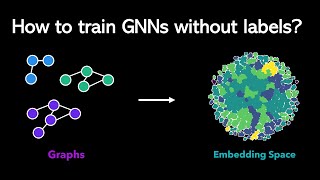
Self-/Unsupervised GNN Training
DeepFindr
Contrastive Learning in PyTorch - Part 1: Introduction
DeepFindr
Contrastive Learning in PyTorch - Part 2: CL on Point Clouds
DeepFindr
State of AI 2022 - My Highlights
DeepFindr
Equivariant Neural Networks | Part 1/3 - Introduction
DeepFindr
Equivariant Neural Networks | Part 2/3 - Generalized CNNs
DeepFindr
Equivariant Neural Networks | Part 3/3 - Transformers and GNNs
DeepFindr
Personalized Image Generation (using Dreambooth) explained!
DeepFindr
Vision Transformer Quick Guide - Theory and Code in (almost) 15 min
DeepFindr
LoRA explained (and a bit about precision and quantization)
DeepFindr
Dimensionality Reduction Techniques | Introduction and Manifold Learning (1/5)
DeepFindr
Principal Component Analysis (PCA) | Dimensionality Reduction Techniques (2/5)
DeepFindr
Multidimensional Scaling (MDS) | Dimensionality Reduction Techniques (3/5)
DeepFindr
t-distributed Stochastic Neighbor Embedding (t-SNE) | Dimensionality Reduction Techniques (4/5)
DeepFindr
Uniform Manifold Approximation and Projection (UMAP) | Dimensionality Reduction Techniques (5/5)
DeepFindr
More on: Research Methods
View skill →


Related Reads
📰
📰
📰
📰
Follow-up: The ArxivLens Protocol: Transforming Research Nois
Dev.to AI
On July 1, 2026, arXiv will spin out from Cornell University, its home for the past 25 years, to become an independent nonprofit organization. Major funding support from Simons Foundation and Schmidt Sciences. Ditching the red for their website. [N]
Reddit r/MachineLearning
CS-NRRM™ Official Publications: Paper 1 and Paper 2 Are Now Available
Medium · Data Science
Found a potential mistake in an ICLR 2026 blogpost [D]
Reddit r/MachineLearning
Chapters (5)
Introduction
2:58
CFs and Adversarial Attacks
5:15
Generating CFs
7:55
Rashomon effect
9:20
Code
🎓
Tutor Explanation
