Understanding Convolutional Neural Networks | Part 2 / 3 - Wonders of the world CNN with PyTorch

Key Takeaways

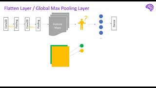
welcome back to the second part of this CNN series in the next minutes we will talk about how we can build and train a CNN in pytorch and how to select the appropriate architecture for our problem remember we wanted to classify images containing the new Seven Wonders of the World with a new network before we start let's quickly have a look at the components we need in our code you might already know that pytorch is an objectoriented deep learning framework this means the functionality is separated into different classes for our use case we mainly need the four four following modules which we will build one after the other a data set that contains our training and test images a data loader that can be used for iterating and batching over the data the actual CNN model which is made up of different neuron Network layers and finally an Optimizer that back propagates the loss to adjust the weights in our model let's have a look at the first block how do we load and use the data set so this is the Google collab notebook we've also used in the first part of this series there we went over how we can visualize the convolution now let's continue here with how we can install pytorch enable GPU and access to data on Google Drive usually you would run a pip install torch and torch Vision to get both python modules torch vision is the module for computer vision tasks from pytorch also make sure under runtime change runtime type you select a GPU session then if you run torch Cuda is available you should get a true which means we can use the GPU so next if we run this cell we can Mount the Google drive to this location and therefore we have to access another URL and enter an authorization code after this is done you will get this message mounted at and if you look at the folder structure here we see we have this new folder here and my data from Google Drive is now stored in this folder so next let's have a look at how we can load the data actually we don't have to do this manually because there's a Pythor function that handles this for us but here we just quickly want to investigate the data we have let's have a look at the folder structure we see we have a test folder and a train folder and inside of these folders We have the different classes and there we have the images for example we have two test images for this wonder and eight train images and in total we have a relatively small data set with only 80 images 10 per label so here we quickly Define the path to our data and we iterate over the files this is not too important but essentially what it does it fills a dictionary with the class type and then a list of of paths that correspond to this class type and now what we will do we randomly select images from this set of different paths and display them to get an overview of our data this is done in this code so I also won't go into detail we will use matplot lip here and here we can see a collection nine images which are randomly selected and we can see the different types so we can already observe a couple of things here first of all we have RGB images with three colored channels our shape is therefore width height and number of channels also we encounter different sizes of the images and later we will have to normalize them additionally as already mentioned we have eight train images per label and two test images per label the pytorch data set class is an abstract representation of a data set and contains at least the get item and Len methods you can inherit from this class to build custom data sets that can be used to index the data at a central place as image data is often a arranged in different folders We can exploit the structure to easily create such a data set with a predefined function so this predefined function I've just talked about is called image folder it's stored in torch Vision data sets image folder and if I hover over this we can see it expects a shape like this one so the folder name corresponds to the class and then we have the collection of different images this is exactly the structure we have here therefore we can use this function we pass it the path to our Ro root of this folder and then this function will create a data set for us and if we investigate this we see we have a data set created from this image folder we have for the training data set 64 data points so images and if I select the sample so the first index I get a tensor like this one which is the image and the second part of this tupal is the label so we will always get a tuple when we index the data that consists of image and label and as you see the labels are automatically converted to numbers instead of the folder name we have a number now here and we can convert them back later and in the back pytorch uses python Imaging library to load these images there's also another thing happening here which are these transforms let's have a look at what is happening there pipelines are used in many places when you enter the area of machine learning the reason for this is that you often had to perform certain pre-processing operations on the data typically executed several times instead instead of executing each of these steps manually a typical approach is to Define such a pipeline that contains these operations in a specific order the advantage of this is that you simply feed in the data into your pipeline and everything is applied automatically for instance we input an arbitrary image and the First Transformation is resizing it to a specific shape after that we for instance convert the image to a tensor which can be used by pytorch pytorch transform compos is doing exactly this task for us whenever we index any of the images in our data set the pre-processing steps will be applied automatically so back in our codes this is what is happening in this composed part we resize all of our images to a shape of 512 by 512 and we use the python Imaging Library interpolation which is specified here and then we convert it to a tensor the same thing happens for our test data set so we have exactly the same code here except we use the test root now as root path for for this data set set next let's talk about the data loader they help us to efficiently load the data and improve the performance of our Optimizer loading the data can become a bottleneck in many deep learning applications imagine you have 1,000 images with a size of 5 mbes if you load and iterate over them you already require 5 GB of memory most standard PCS have 8 or 16 GB so you already occupy a large portion of it data loaders allow us to only load parts of the data so-called batches typically Al you take 32 samples for each batch and train the model with these instead of using all data we Now sample only the small subset for each iteration the optimization procedure is therefore also called stochastic gradient descent as we randomly sample parts of the data it has been shown that this actually converges even faster to the minimum of our loss function in most cases Furthermore with data lootus you can for instance Shuffle the provided data set paralyze the data loading or cat the data after pre-processing to speed up the loading times so overall a very useful class that simplifies the training for us so we can create those data loaders using torch utils data data loader what we do here is we simply pass the data set so the train and test data set we will create a train data loader and the test data loader and we specify Shuffle true which means when we iterate over the data it will be randomly selected or shuffled and we choose a batch size of eight here because we have a relatively small data set so now that the data is ready let's build the CNN model there's always the question how to build such a new network how many layers to use which filter size luckily there are several rules of thumb to simplify the initial steps for us first of all building a model is a sequential process that means most of the time the first model will be further improved as we get experience with our problem therefore simply start with a basic CNN structure for this you can follow one of the two common patterns either stacking pairs of con flare and pooling layer or stacking two con flers and one pooling layer for the filters select odd sizes such as 3x3 the reason for this is that these shapes always have a centered pixel that preserves the location of the activation after filtering start with smaller filters to capture local features such as edges and optionally increase the size in the higher layers of the network generally smaller filters such as 3x3 should always be chosen over larger filters the number of channels should be low in the first layers and then increase as the network gets deeper the reason for this is that we want to capture more high level features in the higher layers and therefore we need multiple feature Maps the low-level features like edges are not so variant and we can start with only a few channels also the pooling layers compress our filtered representations and we need more channels to avoid an information bottleneck using padding is generally recommended first of all because you simply maintain the size of your image but also because you keep the information at the border of the image especially if you want to build very deep cnns it is important to keep the dimension because otherwise the size would reduce very quickly and you couldn't stack any further layers for the pooling layers we can simply use a 2x2 or 3x3 kernel and Max pooling as this works well in most architectures once we have a basic model we play around with the complexity by adding layers of course it is also recommended to get inspired by other popular architectures that performed well on Baseline data sets we will have a look at some of those in a second finally you should also tune the basic neural network parameters such as the learning rate or the activation functions so now that we know how to start with a CNN let's have a look at the Baseline model I created so you can create a CNN simply by inheriting from this neur network module from torch and basically it's always the same pattern you have an init function where you define your layers and you have a forward function which will be called when we feed the data into the network in the init function we have this pattern so we have two conflict layers one pool layer another two con layers and one more pool and after that we have the fully connected part which means we have the classifier here and there we have three linear layers one that takes the input of the last pooling layer and converts it to 12 120 neurons and then we transformed it to a smaller size and finally we have eight output units which stand for the eight classes we have in a forward function we simply stack the layers like this and X is our input image which will be first fed into the first convolution then an activation function reload activation then the second convolution another activation and then the pooling and the same happens for the second stack of these filters and after that we apply flattening I will talk in a second about how this works and then we pass the data further through our fully connected layers until we end up with the output of eight classes so we can have a look at the structure again here we get all the parameters summ ized we use a stride of one and a padding of one we start with three input channels which are red green and blue and then we apply five filters which means we get five feature maps and then these five feature Maps will be further filtered with 10 filters so we get 10 feature maps and so on until we have 30 feature maps in the final layer and we use a kernel size of three in those which means we have 3x3 filters and here we have a current size of five which means we have 5x5 filters and we use padding for both of these I also quickly wanted to visualize the use of flattening operations what it does is pretty simple once we went through the feature extraction so our con pool pattern we observe several two-dimensional feature Maps now how do we pass them into the input layer of a den n network there are mainly two approaches to do this the first option is to reshape the feature map to a one-dimensional vector on other terms we flaten the feature map this means we convert The Matrix to an array by taking each row or column and pending it the length of this array is then equal to the number of neurons in the input layer of the dense Network the second option is global pooling which is compressing the final representation basically it's just another pooling operation that converts our Matrix to a single value this means we take the mean or Max of a complete feature map that's why it's called Global typically if you use Global Max pooling you only have one fully connected layer which outputs your prediction in fact the global pooling layers can also completely replace the fully connected layers in the CNN if we have the same number of feature Maps as output classes in the last convolutional layer we can apply Max pooling and directly use the global pooling values with soft Max for our prediction so there's also another option how to build a CNN using the sequential module this simply means we separate the layers with a comma and we we pass them to the sequential module and we can do this separated for the CNN and the classifier or do it all together and the Advantage is that if we call the function we simply can use this sequential thing and additionally we also don't have to Define variables as we did it here and we also don't have to pass everything manually here this makes it a little bit more compressed and easier to read now we only need one more thing which is the optimizer that adjusts the network parameters to minimize the loss I won't go into detail on how the optimizer and the loss work but I quickly want to mention them here a common choice for the optimizer is Adam which stands for adaptive moment estimation it is an advanced optimization algorithm that uses gradients to iteratively adjust the weights of the network as loss function we will use the cross entropy loss which can be used to calculate the difference between two probability distributions what are the probability distributions in our case on one hand we have the predictions of our model after applying the soft Max these are the probabilities for the different classes on the other hand we have the CR truth which is the true class of an image with a probability of one so 100% the loss decreases when our network not only predicts the right class but if the prediction also has a high probability close to 100 so here we Define our loss function the cross entropy loss and also our Optimizer which is adom and we need to pass the parameters of our Network which we defined here to this Optimizer in order to be able to optimize the weights of this network we choose a learning rate of 0.0 01 which is relatively small and then we continue to train our model I created this train model function and basically all it does is iterating over the train loader which contains the iterator for our data set and in this Loop we basically load the the batch we put it to the GPU and we input it to our model back propagate the loss and adjust the weights and this is happening in the Loop several times we iterate over the data set and I also print statistics so the train accuracy and the losses for train and test therefore I also calculate the test loss and therefore I have a couple of additional functions here our model currently outputs eight classes and we will use the class with the highest probability so we will apply softmax and then we select the class using arcmax with the highest probability so here's an example we train 14 EPO here I also added early stopping which means once the test loss is not getting better than the current best loss we increase the early stopping counter once this counter exceeds the patience we have which is for example two EPO uh we finish or terminate the training for example here we can see the test loss the smallest loss was 1.49 and here you can see the loss increases again a bit fit and starts to get worse and that's the point where we abort the training to avoid overfitting and here you can see the train loss also decreases from 2.10 to almost 0.4 and in a training data set we get an accuracy of 0.87 so 87.5% in the test data set we only get around 50% accuracy so we can also visualize how the losses behave using this function we calculate the accuracy as how many predictions are correct if the label that our model predicts matches the ground truth of the model we say it's correct and then we sum up all the correct ones and divide them by the total number of samples we used we can visualize the loss like here and this would basically be the point with the lowest loss and actually we should use the weights of the model at this point so we should always store them I didn't do it here so for this I will use the last weights of the model but ideally you should always use the ones with the lowest loss now this code selects the next batch of our test data and then inputs this badge to our model to get the predictions and after applying softmax we will also get the probabilities for these predictions we can use them now to calculate the classes for instance so we set the batch size is eight that's why we have eight values here these are the probability values that our model predicts and if we select The Arc Max again so the class with the highest probability uh we end up with this the first one is the outputs which means the predictions of our model and the second one are the true labels so you see we predict two and the crown truth is also two and so on and we can also visualize this so whenever the text above the image is green it's a correct prediction and when it's red it's a wrong prediction and I also put the probability values after applying the soft Max here so we can see how certain the model is about its prediction and this is for one test batch so for one set of unseen images and we can see the pyramids do pretty well we have 79% certainty here and the same for this image but we see overall the model is not performing very well it's also not very certain about the predictions this corresponds to the result we got up here which is we have around 50% correct predictions and that's basically what we get here so now the question is can we do better how can we improve our model one thing to consider when training a neur network is always how much data do we have as you know we have a relatively small data set only 80 images 10 for each class data augmentation allows us to enlarge our data set without searching for new images therefore we make Minor Adjustments to images we already have a simple possib ility is to select only parts of an image this is also called cropping another technique is to flip the image horizontally or vertically if different colors occur in our data set we can also play around with the color values such as gray scaling alternatively we can also rotate the image with a certain decree these are just some simple examples we can easily add to our pre-processing pipeline note that there exist also more Advanced Techniques to generate more data such as general ative adversarial networks but for our simple example we will stick with these basic augmentation techniques so in the code we can use the transforms module we already know because there are different classes such as random rotation and here we pass the degree so this will randomly rotate the image by 10° or we can use this random resized crop we pass in the image size to which our image will be resized after cropping and it will randomly crop out parts of the image according to the scale information and then resize them to our original shape also we can randomly for example horizontally flip the image so there are many other possibilities and you might have a look into this transforms module because there are a lot of Transformations we can easily apply here in our pre-processing pipeline so therefore I create a new augumented train data set and therefore I also create a new train load that uses this augumented train data set and note we only want to adjust the train data set and not modify our test images of course now here we can have a look at a sample if I take the first image of the first batch uh we can see we have a cropped out part let's run this again we can see it's slightly rotated maybe one more so this is rotated as well this introduces a little bit of variance in our image so if we train this again and here I disabled early stopping because there was less overfitting for this model we can see we managed to get up to around 0.56 and here you can see it's also not not overfitting and if we again display the images as we did it before we can unfortunately see that the predictions did not really improve I can run this again with a new batch so still the pyramids are performing quite well we have better values certainty values for some things like the Coliseum in Rome has now very good values but overall it's not perfect yet to be honest but there's room to improve especially in the next part we will uh use transfer learning to further improve our results but now let's have a look at further CNN architectures so now we have trained our Baseline CNN architecture and played around with data augmentation to improve the results but what if our model is still not performing as good as we expected how should we change it well you don't always have to reinvent the wheel there have been many Publications on different approaches to create the CNN architecture with the best results and still today the modules are continuously improving better accuracy less parameters and more efficient feature extraction these models are typically compared on the image net data set which is a large collection of labeled images all of these CNN can also be loaded in pytorch the this means you can also use one of these well tested architectures and don't have to come up with your own design and actually we will also do this in the last part of the series when we talk about transfer learning in the following I quickly want to explain the ideas behind a couple of popular CNN architectes there exists so many different Publications that I could make a complete series on different models but this is not the focus here I just want to show you some examples so you get a feeling for what the experts in this area did let's start with one of the first popular architectures alexnet it consists of eight layers five of them are convolutional layers in total it has 60 million parameters and achieved a 47.1 accuracy on the image net data set so overall not many new things here we can see that the feature extraction part is a mix of convolution and pooling layers as well as a couple of fully connected layers similar as we did it in our Baseline model alexnet uses the reu activation function and overlapping pooling furthermore more the first two fully connected layers used dropouts let's have a look at what dropouts are the basic idea of dropouts is to randomly drop out units so neurons in the network during the training as a result the network learns to not focus on one specific feature but rather use all available information in a distributed form dropouts prevent overfitting and make the model generalize better they are a regularization technique dropouts can also be seen as an ensemble approach as they average over a set of possible sub networks this technique is applied in many newer networks let's move on to the next popular CNN architecture stacking layers allows us to capture highlevel features by combining the feature maps of different filters so what happens when we stack many layers say for example 100 when the CNN gets very deep the gradients have to back propagate many layers and many multiplications are performed as a result the gradients get very small this is also known as Vanishing gradients problem and usually the performance decreases when too many layers are added residual blocks are simply connections that Skip One or multiple layers in this example all neurons of the first hidden layer are for instance connected to the third hidden layer you can see it as a shortcut in a network as a result the gradients can smoothly flow over many layers without getting too small neur networks that use this mechanism are usually called res Nets the basic idea of these skip connections is used and extended in many pop large CNN architectures one prominent example is resnet 50 which has 50 layers and 26 million parameters with 75.8% it performs significantly better on the imag net data set compared to alexnet you can see how the shortcut connections are added in the identity block another thing is that this architecture has only one fully connected layer and uses Global pooling which has been presented earlier there are further Advanced Techniques used in different CNN architectures but it would be simply too extensive to capture all of them in this video series however I want to talk about one more thing that was also used in reset 50 as you might know data should be normalized when we feed it into a new network this can be achieved by for instance standard scaling or minmax scaling have you ever wondered why this normalization is done if the data is not normalized the optimization of the loss function is more complex especially if the ranges of the input data are different among the features some parameters will be emphasized more than others as a result the training of our Network takes longer through normalization for instance converting the input distribution to a mean of zero and variance of one we ensure that we end up with a smooth optimization function but why should we stop with normalization after the input layer in a network many activation values flow from layer to layer and it might happen that the mean and variance of these values changes this phenomenon is called internal covariant shift if these shift are not corrected the stochastic gradient descent would need to learn the shift as mean and standard deviation as additional parameters batch normalization simply normalizes the activation values so the input values for the next layer using the mean and standard deviation of the current batch this means we get a mean of zero and a variance of one this ensures that the distribution of inputs will not change in the network overall the optimization is smoother because the network doesn't need to learn the shift in the distribution from l layer to layer besides the presented alexnet and rest net there exist many other variants of CNN architectures for a great overview I can recommend the website papers with code which provides a large collection of different CNN approaches other popular architectures are for instance efficient Nets res next or Inception in the computer vision area there are also many other applications where the CNN pattern with convolutions and pooling is used Worth to mention are for instance convolutional order encoders and an interesting design pattern that is used for many applications they are able to learn compressed representations of the input image another example are so-called units that can be used for image segmentation this means they are able to automatically extract parts from images which is commonly used in medical imaging finally another interesting design are generative adversarial networks or short Gans they also use the basic CNN layers and basically consist of networks that try to battle each other one network creates images the other network evaluates them there's a website called this person does not exist.com which shows how powerful this architecture can be all the images you find when refreshing the page are generated with a again and the person that is displayed does not actually exists but is randomly created by the neuron Network I also encountered some examples where the generation is not perfect I just wanted to mention a couple of variants in the basic CNN idea for complete this here there are many things you can do with ner networks I didn't use it for this video series but generally if you start a new pytorch project I can recommend to use pytorch lightning which is nothing more than organized pytorch code this makes it easier to train and play around with the model as well as maintaining the code you don't need to worry about selecting the Cuda device early stopping logging or iterating of the appx as this is all done by pie torch lightning plus you don't lose any flexibility and keep pure P torch that's it for this part in the next part we will get familiar with transfer learning and further improve the model finally we will also have a look at explainable AI to better understand our CNN thanks for watching feel free to leave comments if you have questions see you in the next part