The practice of doing performance analysis/optimization with TensorRT-LLM

Key Takeaways

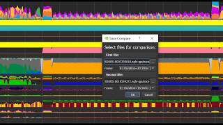
Good morning. Hey. Hi everyone, thank you for tuning in. If you've been here before, welcome back. And if you're here for the first time, thank you for joining. Today we're going to have a session on the practice of doing performance analysis and optimization with Tensor RTLM. We're joined by two awesome speakers. First up will be Caillou, a comput architect engineer who's actively contributing to Tensor TLM and focusing on general performance. And then we'll hear from Cyrus, an AI developer technology engineer who's actively working on LLM inference framework kernel performance analysis and optimization. Caillou, take it away. >> Thank you. Hi everyone. So today I'm talk about uh so me and Sarah we are going to talk about the practice of doing performance analysis and optimization with tensard DRM and um we have agenda that uh have five parts. So I'm going to take the first three parts that includes the use um some of the useful tools and and tips for performance analysis and do some um actual um practice on optimizing that on the system level and Sarah is going to take um take uh introduce on how uh usual codraph kuda kernel analysis is is being done and um how optimization is going down in the tens. are TR. So um I think today I'm not going to uh introduce too many details on how those optimization is being landed into TRD but um more focused on we're going to focus more on the um how we are going to use those tools and how how are those tools and the functionalities that are provided by Tanzard going to help with the performance analysis. So let's let's get started. Um so first of all I'm I want to share um the most mostly used example command that we used for um debugging and for benchmark um tens in a very typical um scenario. And so this is a uh a command when you are trying to use the bench to benchmark tensm and when you are trying to use an assist profile to um profile the time timeline that um how the bench is um doing the benchmark and you could also you you could certainly replace the TDM bench command with the TDM serve command. Um but um the profile idea is the same. So it basically use uses several different chases. It uses CUDA profiler API and um it enables some of the uh environment variables pro provided by Tenszar DRM to um to to get more information and to have a better way of um debugging and and um find find out more information on how um Tanzar DRM is um is implemented and how it uh will functionally work. So you you could also refer refer to the document um that uh I put in the in the link but um but but I I I'll I'll go through uh some of the most important environment variables and arguments that are involved in this command. So the first three um helpful environ variable includes um TR profile start stop um TRM MVTX debug and TRM profile record GC. So the start the first one the TRM profile start stop um will help you to only correct specific inference in iterations um for example from from A to B like from one to 100 or uh from 100 to 200. So what's that going to do is that will help you to narrow down the focused uh performance hotspot. For example, if you um so if if you just want to see um how the program is running when GPU step is between uh 100 and 200 um or if you if you are end to end for example if your end to end program is running like for one hour or two hour and you cannot actually just uh profile the entire one hour um process of the benchmark then you can use this way to reduce the the profile size and to only focus the on the part that you are interested. So you could you could use this environment variable and the RDM will only profile the specific range of the iterations and um it only it only take effect when you also append um - C uh CUDA pro CUDA profiler API um which enables the u programming a programming way of of NS profile command um and that and and and the corrected timeline will just be uh narrowed down to a a-b and the second uh environment variable is uh TRM MVTX debug and that one actually just uh enable more MVTS markers for better debugging because we have um prepared um many MVTS markers in the in the system on different locations and if you uh enable this environment variable that those uh those markers will be visible and um also it include we we we've added a environment variable called DM profile record GC. So if you set that one to one that means you can enable the Python GC um and VTS markers um for the um for the users who want to get hints when um when the time is actually spent on GC and uh the there's a a snapshot the the di diagram is actually uh showing how the Python GC markers are going to show on the on the on the timeline. Um for this in this case it takes almost four milliseconds. Um and this way you can actually know um when is waiting uh when when the Python GC is actually taking the um take taking the CPU work. So um moving further there's a one one more very helpful and um I actually use it a lot. um profile option but that this one is actually implemented by NSA profile and uh it's called Python Jio. So this one enables Python global inter interpreter lock uh aka the go uh markers together with the other informations um when you are using commands like anis profile and you I I usually enable it together with cuda and vtx and you could also refer to the official um documentation of um profile to to see more information and this um this argument is also very helpful and and and being uh heavily used when I'm debugging the performance of tens when it when when it um happens I mean when you want to take a look at the performance status of the system. So especially when you are analyzing the the Python behavior on CPU because it actually tells you how um Python is occupying the resources by acquiring the geo and because sometimes if you see that a specific MVTS marker um is very long, you might be uh confused that why it took took so long and sometimes um it in fact does not take such a long time to just uh for CPU to to finish the operation. But most of the time is that um CPU is actually waiting for Jio um for on the on the other thread. And I I also put an example here. And this is this one is a very typical example when one thread is waiting for for another thread to release the geo. And you could see that um the on on on the green bar that um the the darker green bar is uh with the text uh holding gio on it is the one that um the the corresponding thread is actually holding the geo. Um while the other the other thread on on that on that process um are waiting for the for that specific thread to release the geo. And that's the basically what um how pyon go is is is working um in python. So um this is very helpful because uh tenzard the most most part of tensard API and the core library is implemented on python and um python have this since python has this specific go mechanism um we need uh we need such functionality to to decide um where actually the the hotspot is um so based on some this some of this um brief uh introduction on how uh those tools are used and how uh we can profile and do some performance analysis on it. um uh we can uh moving we can we can moving one one step forward and um take a look at overall implementation and then I'm going to uh introduce um two specific examples on how we use those tools to analyze the the performance and try optimize it. So the overall implementation of current TRDM um on system level is that we we I mean th this is a simplified model but um it explains um how it basically work. So we have mostly two processes. Um the main process is going to be the the process that um handles the server and and handles the user interface. So it it receives the request from the user and um it also uh will be responsible for spawning a MPI process and then we're going to have a worker process. Um so those two uh process are are the major processes that are handling the the most of the Python implementation on a on a in TRTM. And when the request is is re is reaching the main process um it will be uh firstly um just directly um given to a to the worker process through interprocess communication and also the main process is going to um spawn uh create different uh stress and the worker process are going to create different stress as Well um and so the worker process will create two uh one important um thread called a weight response thread and uh then when the request is is um uh is is passed to the pi executor the uh pi scooter will launch um the specific executor of um the um the the actual implementation of the scooter such as pi scooter or cpv time scooter and if um if if the request is is um uh given to the pi scooter it it will uh launch kernels and it will finish the calculation needed and um for example for for lm's output ids are going to be uh generated and responses are going to be generated by and DN and when responses are generated um the first thing is that we're going to um we're going to pass it pass them the generated responses to the await response helper um and that process is a communication within the process and the await the the thing that await response worker or helper is is trying to do is that it well uh forward responses to back to the main process. So you could see that there's one more um um interprocess communication and the await response helper will uh give the responses of the responses to dispatch result task and the dispatch result task is another thread uh that is created by the main thread and it will be responsible for um giving those responses back to the donizer and Um uh on another case when user is enabling the D tokenizer, it will give the responses to the D tokenizer and the D tokenizer is going to do its work and converting the the the token ids to um to string and it will uh and afterwards it will the main process will also create the final responses like for example for TM serve it will um give the response responses back to the open API server which uh is built based on the fast API server in in tensor DRM and um all those responses will go back to the user in the as the as the last stop of um of its um life circle. So this is the overall implementation and if you are trying to profile um tensor DRM you are going to see something interesting because um the the profile or or the timeline you're going to see is that um it will be very similar or or or um it will reflect how it work as as I just mentioned and you could see some interesting details. else based uh based on that and this is an very um so this is an example of um what you will see when you are trying to benchmark and profile TRDM um using the command I mentioned earlier and this one is is a overview um back to the version of 0.20.0 zero RC1 because I I use that uh version to to demonstrate um what it was like before we landing some optimization and um and by the way you can find the latest version and on on GitHub and we we are uh currently um um preparing 1.0 zero. Um the and we we published some release candidate version and we when you are benchmark and providing the uh implementation on the latest uh version, you could expect something different than this one I just mentioned. And um so back to the timeline you could see that there are several different processes and and um threads and we we could uh roughly um mirroring the the the processes and and threads back to the previous page. And um we have Poder, we have a weight response helper, we have uh the dis dispatch result task and and the detonizer. And this only reflect the um the the second part of the life cycle of of a response of a response because I I skipped part when the response gets created. So um you could see that there I I marked several annotation or u the red boxes there on the on the graph and um it means it it it is trying to explain um what's happening to that responses as at that time and um for example when the responses are created on the pcuer um it's going to be serialized and and des serialized when when we are we are doing round up or get for uh features like attention DP and um then it goes to uh await response helper which is a in char uh process communication and um the await response helper will send all those responses to to another process uh which is a interprocess communication and which introduce a um serializ iz a set of serialization and des serialization and also of course a a a send um and when the dispatch result task receive the the responses it's going to uh forward that one to to uh to the d tokenizer and the d tokenizer is going to I I annotated as uh prepare outputs but it's actually doing something like um d tokenizing the the tokens and and um and prepare output uh open AI server output for for the uh for the final for the endpoint users. So we could actually uh see uh um the the implementation idea of tons by just profiling and uh benchmark and profiling the the models and um and we could actually observe the the way that how it's done um by um inspecting the the timeline and also uh so we if we if we Um take a look at take a look at this graph. We could see that um there are several parts that looks confusing and um for example um if we take a look at this part specifically you could see that um those responses are >> Caillou I think we've got a couple of questions. So let's take a moment real quick before we go to the next slide to answer one of them >> and he'll bring it up on screen for you. Um, let me see. Yeah, that's a that's a very good question and I think uh currently we so um in in ter of of a media we we are using uh several different slum clusters and that part was actually take care of the by take care by the slum clusters and the slum clusters is going to be responsible for um things like doing the actual um SP I mean and also together with the MPI rivalry they're going to be responsible for the actual implementation of the spawn and and and the the process affinity and um and we rely on uh the infrastructure to um to guarantee the performance of um of like something like um interprocess communication um and and and and that's that's also the same for uh for multiGPU for multi for multiGPO uh communication and also between uh multi-nose communication that should be the same. >> Thank you. Okay, I'll I'll move on if that um address the question and feel free to let us know if if uh I'm I'm not being clear. So um so um as as I was uh discussing so um this one here is all those responses have been uh experienced different stages of serialization derization and and then serializ serialize again and then d serialize again and there's one um set of duplicated derialize and serialize And so we were seeing the same um issues there and we were thinking about how can we like remove the duplicated serialization and deralization. Um and we uh we did some analysis and we optimized the the second part of the derelization serialization by delaying the der the the second d serialization to a later stage. Um that helps on two aspects. Uh one is on um one one is that um it saves some some time which will benefits TDFD and to the second advantage is is is that um it will also uh reduce the size when we are doing the interprocess communication and that will make the communication like uh like the MPI or MPI I um um uh broadcast faster. So that one is one of the optimization we um landed in um when we are seeing this uh profile results and another example is um is very usual is a very usual case. So on some of the cases on especially for streaming mode um we usually assume make the assumption that um each iteration has to return responses for every request that um includes the token generated on that iteration. Um so for example when streaming is enabled and when um the output length of of the of of the specific prompt is 10 then um 10 token will be generated and on each uh GPU step or or each GPU iteration um one token is going to be returned I mean one response one response is going to be returned for every single token uh single token. So um that will so when the batch size is very large that will actually lead to a very heavy CPU um operation and for C for for the CPU work and that could take a lot of time and um some we have observed actually some extreme cases when we are supporting the scenarios when device size is very large and the that is when CPU cannot even finish all those operations before um the next GPU iteration starts and that could significantly affect the streaming performance and the final throughput um and and this corresponds to the to this part on the on the on the diagram I shared earlier. So in order to resolve that we uh introduced a uh stream interval feature and in so the logic of that feature is that instead of handling all responses on each iteration uh we allow users to specify a uh argument called stream interval and you can set it to n and that end well means that uh the responses will be handled and returned every n iteration. ations. Um that way on each iteration um the output ID itself will still be generated by by GPU and and being uh by uh calculated by by GPU but um it won't be uh returned to users immediately um except for for the first token for for for DDFD. Um however the tokens will uh be accumulated for any iterations and and um one and and afterwards when responses one response is created to handle those and generated uh tokens and this actually helps uh reduce the pressure on CPU side and it give more uh chances and more time for for the CPU to catch up uh the the work that GPU is doing because um the CPU has to be faster than GPU otherwise GPU will be waiting for a CPU and that will lead to bubble on the on the on the CUDA stream. So um so in in order in order to um see the effect effect of of our optimization uh this is an uh I put a diagram here after the uh the the optimization and and when uh when the user on this case it should be 16 and when a user is specifying um a um specific stream interval. Um all those uh responses handling work like tokenization, detoization and preparing um open API server outposts are going to be um separated to to uh be limited to uh specific iterations and it will just give the CPU more time to to catch up. And um and this one is uh useful for for stream uh streaming performance. And it it is also uh very um um recommended and um and also uh the the the the impact the influence can be clearly uh observed on an profile when you are uh profiling the the program and yeah I think that's uh all for my part and um yeah >> all right thank Thank you, Caillou. Before we move on to Cyrus's part, let's answer a couple more questions. >> So, we have a question on multiGPU profiling. >> Uh, how do your profiling and optimization do change when scaling from a single especially regarding graph fusion cross devices? Yeah, that's a very good uh question as well. And um for this one, it actually so uh let me just quickly go to the previous page. So um so this command actually it won't change too much but uh the the the case that you want to uh be careful is that um the uh since this is one this this command is only for one one process. So if you are going to uh for example if uh if you're going to profile a my GPU program using this command you may want to um separate different um oh sorry separate different uh profile file names and uh so that it won't uh trying to write the the profile the timeline profile to uh to uh to the same to the same file uh which will lead to confict. Other than that, I think all those commands can uh all those arguments can be just reused and they are common between single GPU, multiGPU and multi nodes. >> All right. And then one more question for you. >> Uh which did you Yeah. Uh we so uh as a as a very quick um kind of like kind of like a verification uh we can just use TDF and ITL that is 10 uh um 10 to the first token and uh in the token latency and we and also the the overall um output throughput output token throughput and that those metrics will uh will be used to measure most of the uh performance improvements we we we are doing because uh most uh clients well what most clients will care is is DDL and um and final final and um we als we use those specific metrics for um for those uh performance optimization including the DC serializ optimization. All right, great. Looks like those are all the questions we have for now. Um, let's move on to hearing from Cyrus. >> Thank for sharing the runtime performance analysis and optimizations. So, >> so I will share the CUDA kernel performance analysis and optimization with the several like real cases we have been doing the kernel optimizations in the uh tens. So the first step to analyze the CUDA kernels is to use the NSAT system the NISS to locate the slow kernels. So uh in the NCS we here we use the DCR1 IP8 block scale quant kernel on H200 which was uh which um on the version 0.19 where we found this like in the NC there's a uh there's like if you expand the total kernel times you can there's a mappings of like each turn each kernel's the percentage of each kernel's took. So in in this example we can see this like scale one multiply 128 kernel which is the IP8 quant quantization kernel took took about like 12.8 eight in the total time and also in the timeline we could see like this uh there are they are some sometimes to be very long like this kernel before the matrix multiplications which is very strange because the quant kernel is a element wise kernel which should be very small and quick. So in this case we know like where this kind of may need might need to be optimized. Uh then after locating the slow kernels we need the more details and more detailed informations and the analysis of these kernels. So we need to use another tool which is Nvidia inset compute the NCU to analyze the kernel performances. So NCU is an interactive CUDA kernel profiler then that provides DQ performance metrics and API debuggings for the CUDA applications and the kernels. So the best practice using the NCU to profile a kernel is first to isolate out the kernel from the tensm and then use the NCU to uh generate the profiler reports for that. So when we open the NCU report there will be we we will see several kernels with its name and its duration. So here we have like six kernels and they are actually all the same kernel but with two different problem problem sizes. So it means like each kernels have three identical code profiles. To see the details of the profile we can just double click one kernel and it will jump lead us to the like the details tab. So on the in the details tab on the top right in the view section in the view button clicks the expand sections and it will show all the details of the uh kernel kernel performances. So the there are several very helpful like sections and when analyzing the kernel performances at the top of the details tab is the GPU throughput table where which shows the compute and the memory throughput. So with this data we could identify whether this kernel is memory bound, compute bound or latency bound. So in this example we could see both the computer and the memory throughput are very low which means it which indicates it is a latency bound kernel. Lat bound kernel usually happens when the kernel is small which can confirms our assumptions through in the NCU. So the next helpful table we usually use is the warp scheduleuler statistics table. So the first line is the uh GPU max warp peruler which is 16 because uh in the GPU design one streaming multiprocessor one SM has four Wululer and one SM has at most 248 threads and one warp has 32 threads. Four, one warp scheduleuler has at most 16 warps and the on the second row is theoretical like warps per scheduleuler which means like how in in the way how many actual warps can be in in one of this kernel. So in this case it is 16 means is means it can reach the max warp peruler. So the third line shows the real active works per scheduleuler which is in our case is only 1.99. So compared with the 16 theoretical value it shows like the the SMS is very underutilized. So so the parallelism of this kernel is not very enough. The third the next useful table is the web sty chart. So the stop in GPU usually means like the warp stops and the wait for some processes to finish before they can continue to work. Uh there are several there are multiple reasons of of the causes to the stall and the NCUS can helps to list all kinds of like stalls and analyze their performances. In this uh example, we could see the most significant stall is the styong scoreboard. Uh styong scoreboard means like the work is stalled waiting for uh global or local memory read and write. So to be more specific, there are some operations in the inside the kernel which is waiting for the memory read from the global memory in this case which makes the GPU not efficient. So the next next table in the occup is the occupancy table. Occupancy is the ratio of the number of active warps per SM to the max maximum number of possible active warps. So higher you usually higher occupancies doesn't always result in the higher performances. However, low low per occupancy always reduce the ability to hide uh latencies resulting in the overall performance degradation. So we could see like in the uh table the occupancy of this kernel is only 12 12.39% compared with the theoretical 100% occupancy. So this indicates the SM is very underutilized which is like Chris which synced with the uh previous slides the uh warp scheduling statistic table and on the right side is the block limit calculator uh which is used to calculate the block limit per SM to reach the max occupancy. So we will cover this this part this this part later in the slides. And uh there's also another type mean uh another type in the NCU report which is the source type. So NCU can help correlate assembly uh the SAS codes with high level codes such as the CUDA C codes. Uh in addition it displays the instruction correlated matrix to help pinpoint the performance problems in the code. So in this example we can see it highlights the code that causes the long scoreboard with this like yellow uh triangle sign on the right is is like a uh the this this part of code is calling the 80 99% of the long skill board and going back to the kernel to the left is it shows the which kernel is having this problem. So we could see like the problem line depends on it previous line L's data the input frag the input frag is actually read uh re read it from the global memory of the input line. So regarding reading from global memory is a long latency operations in GPU. So the war needs to wait till the read ends. This cause this is the reason why the long score both happens and uh and we can also notice there is a for loop with like a four iterations. So it means like each iteration the this stuff happens in each iterations. So these are all the helpful uh tools we helpful matrix and tables we we like we use while doing while reading the NC reports. And next we will uh I will discuss about how to how do we optimize the this kernel uh based on the analysis is on the NC reports. So the first thing is to reduce the star long scoreboard. So the left graph shows like the logics of the uh original code workflow. So each computation depends on its previous global memory rate and uh all the occup uh operations are done in serial in done in serial. So to reduce the long score B we could split the split the global memory read and the computation to two different loops. So it can achieve better memory reads and also it can overlaps the reads and the computation to make it to make it a pipeline instead of instead of uh serial operation. In the meantime we can use the vectorized the read to accelerate the reading from the global memory. For example in this case the input data type is 16 bit either BF16 or uh FP16. So we could use the already provided CUDA uh 16 bit vector which is the FP162 or BF162 vector to transfer the uh to to transfer the 16 bit rate to the 32bit rate. It means like uh uh when reading we we're actually reading two two 16 bits and combine them to be a 32bit read. So it so it can save the instructions because the LGD16 read instruction will be converted to the LGD32 reading instruction. So LGD LG is actually a SAS command meaning like a reading from global memory. So we are saving the instructions and as well as we are uh uh our read will be more coal. So after the co change the new code will be look like this and the the next the second optimization will be uh how to increase the occupancy. So uh uh in the occupancy table the NCU provides the maximum maximum number of the threat blocks that can be resident on one SM based on different limits. For example, we can see the limited by the registers number, the share memory size, the warp number. So in in other words, the minimum value of the of all these values is the maximum value one SM can should have to reach the max occupancy. So in this example, this value is eight. And the in the original uh in the original launching in our original codes when launching the kernel we are actually only launching the number of SMS which is 138 and 138 132 thread blocks. Uh but we from this table we know we should have like eight multiply number of SMS which is 156 thread blocks. So with this simple like uh change we can see that the now uh now the occupancy has increased from like 12 339% to the 73.2% 2% which means like we're getting actually five times more or six times more occupancies uh assigning more blocks to per SMS could assign like more works to theuler so they so the schedulers can see more add works when that when they are scheduling so it can fully utilize the GPUs so so after the optimizations let's see the result of the optimization So compared with the original kernel, we could see the optimized kernel can have six time sixx more occupancy, fivex less kernel latency, uh 4x more compute throughput as we can see in the uh uh blue and green chart, 2.5x less long scoreboard. So projecting this C kernel speed apps to back to the end to end uh NC reports the we could see like the new uh this new optimized kernel now only 3.4% in the over in the total kernel times which means like we are reaching around 9% end to end speed up. Yeah, the there's another kernel optimization which is which is usually the kernel fusion. So which means like fuse several kernels into one kernel. Here we will use the fuse the gated MLP as an example. Uh gated MLP layer is a very common layer in the large language models which uh happens after the attention layers. So the the workflow of the original gated MLP is the input X will be will be sent to two different matrix multiplications. The fully connected FC and the gated app projection GitHub. uh the result of the FC kernel will be sent to the uh CU activation and the the result and the uh result of the activation will have the the inner product with the gated result of the gated up projection and then the result will go through one more layers which is the another matrix multiplication which is the dump projection uh down projection uh J So from this workflow we could see like the uh FC and the G app jams actually are independ independent they are two two independent jams and they they use the same inputs. So it is like a so it is very helpful if we can concatenate the input and the weight will do to merge to fuse these two two jams into one large jam. So, so after we do this, the the new workflow will be shown as at the right which which is like the the input X will be passed into this fuse the new fused gated app uh jam which which the input X will be duplicated and the weight of the uh FC and the gate app will be concatenated and after this gated app projection uh projection jammed they will go to the new new activation kernel which is the swoop kernel. So the workflow of this swoop kernel uh uh is like the input x will be uh splitted according to the last dimension to uh to convert them back to the FC and the gated app kernel. So uh the result the FC will be passed to the C loop as the original like uh get get up uh original get MLP loops and the the result of the CU and the gate and the gate will do the inner productions and and this is the same and the result will go to the D projection. So uh so what is the benefits of doing this kind of fusions? The first is like the uh memory bandwidth is the memory bandwidth optimizations. So we could see in the original implementations uh it needs two separate to read and read from the global memories global memories because usually the input is very large uh tensor. Uh so they will be the the read will be uh passed to FC and get it up. But now we only have one read and write because the weights are concatenated and we are just duplicating the inputs. The second benefits is the kernel launch time overhead reduction. So launching launching a kernel in GPU is not free. It needs some CPU. It needs the CPU to send the launching launching commands. So usually it took about uh two microsconds to 10 microsconds to launch a GPU kernel. So fuse fuse the kernels into one kernel can help reduce the launching launching commands which can help reduce some of the overheads of the causes by the kernel launching. The third is the better compute efficiency efficiency. So the one large gem is usually is faster than two small gems because it has higher first has has higher arithmetic intensity which means it has more flops per bat. Uh secondly it also on modern GPUs for example Mere Hyper and the new black wheel uh it can have better utilizations on the tensor cores because they are it it because the problem shapes are larger. Uh the third point is like it could have better memory coraling patterns uh which which means like uh reading uh one large the reading efficiency will be uh much better than two different smarts. So uh as a result we could see in the N6 report uh the previous original implementation is around 90 89 uh microsconds and with this new op optimization the new time is the um large gem now is like 68 microsconds so we are saving 20 microsconds which is around like 20% more speed up on this fusion and uh this fusated MRP now uh the these screenshots on the NCS are based on the uh old Tensor RT back end on the H100 GPU. Now we have the the Tensm has the new PyTorch uh back ends pass which which we already applied the this fisticated MLP uh fusion by default. Yeah. Yeah. That's my uh today. Yeah. >> Thank you so much. Um, so at this time, if there's any more questions, please drop them in the chat. And then I've seen a couple of people ask about this. We're going to be adding a link to the slides in both the LinkedIn YouTube description. So you'll be able to find that afterwards. It looks like we have a question. Um, how do you decide when to apply or skip fusion? >> Yeah, this is a very good question. So uh usually when we want to do the fusion we we usually do fusions on the small kernels because uh first they are pretty first they are small uh which means um we we usually do kernel fusions based on the kernels like first day it is like uh independent kernel kernels on each GPUs means is it is not a multiGPU kernel for example the or reduce kernel or or g kernel second the kernel they are consecutive This is the small kernel. So it it can be fused to the larger corners or it can uh or or there are several small kernels together. So we can fuse them together. Uh the main benefits of doing this fusions is like reduce the global memory read and write and reduce the kernel launch overheads. Yeah, that's why we that's when we usually do the kernel fusion. It's like when we when we say consecutive small kernels, we do the fusion. Yeah. >> Thank you. Um it looks like that might be all the questions that we've gotten. Okay. Well, if that's all the questions we've had, thank you everyone for joining us and we will see you next time. >> Thank you. Thank you.