Live Day 6- Advance Statistics With Python In Data Science

Key Takeaways

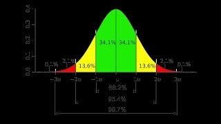
hello guys i hope everybody is able to hear me how are you all i hope you're doing fine absolutely fine we'll just start the session can you hear me nice hello okay perfect so please hit the like button before joining as usual okay uh so today's session we will be continuing the discussion where we have left yesterday and probably i also want to discuss about some of the things uh which i have missed and then we'll try to cover that we'll also try to see some kind of practical examples okay so all those things will probably get covered and yes let's go let's go ahead and probably we'll wait for another five minutes so that ah seven o'clock uh we can start the session right but before going ahead uh i hope everybody has seen my hindi playlist on krishna vlogs channel so you can go ahead and see that also i have started uploading videos on that too okay please make sure that you subscribe that so that you will be able to see those videos also yeah day 5 day 4 resources on day 5 day 4 resources are uploaded i'll just have a look okay i'll just have a look probably uh if i'm able to find it out i will definitely do the necessary changes but it'll take time okay so day five day five guys but if you go down you will be able to find everything over there no now it is not the same resources that is the continuation resources okay so in the next sheet you will be able to find it out right so please make sure that you watch those uh they are uploaded you can go down it is the continuation like this is the same sheet i'm talking about right so here you will be able to see this was day four right and day five we started from here from here right so please uh do that particular part also okay a to b testing becomes now easy right if you know all these conditions yeah let's see i will take an example tomorrow so today is the sixth day sixth day live session shall i use a new sheet let's go ahead and use a new sheet okay so sixth day live session okay so today what all things we are going to discuss okay today uh first of all uh we will continue uh with the discussion where we left so we will solve a chi square problem okay the second thing that i forgot about some of the topics over here is with respect to covariance correlation congratulations ramesh he got an offer from tcs amazing congratulations guys just same congratulation pearson correlation coefficient and the fourth topic that we are going to see is nothing but cpr man rank correlation coefficient right we are we are going to just a second peer men rank correlation coefficient we are going to discuss about this then probably we are also going to see practical implementations okay so we are also going to check out some practical implementation things okay now in this practical implementation we will try to perform z test t test and probably also see how to perform chi square test okay i have taken entire course two days back which entire course are you talking about tamar guys my voice is not low i can hear this in my youtube channel it's quite high okay so i don't think so my voice is low is my voice low is my voice low guys so this is what we are going to discuss guys my voice is full high i can check it out okay my voice is absolutely fine i guess okay so for the people who cannot hear me okay so just try to increase the volume of your laptop or your desktop or use earphones that would be amazing okay okay perfect so many people can actually see this okay this topic uh we will also see f test which is the last topic which is also called as anova test okay the reason why i've kept f-test as large because the calculation will be uh very very uh you know the calculation is quite the calculation is quite complex in that particular case okay now guys i think i've set the volume high so everybody is able to hear many people are able to hear it i guess okay okay guys so let's start uh the first thing first let's go to the chi square test and let's solve a problem uh i hope my energy level is quite high because it is a seven day session you know sometimes you feel low you know the energy becomes low because same thing like uh but the plan is to basically cover everything in such okay so now let's go ahead and let's try to discuss about the chi square test uh chi square test has quite amazing uh problem statements okay so if i really want to discuss about chi square test it is mostly i'll i'll talk about it okay right now so let me just define what is exactly chi square test chi-square test okay so the chi-square test the chi-square test claims about population proportions that basically means if someone asks you krish okay someone ask you in the interview why is chi square test use that why it is used you can just say that it is a non-parametric test test that is performed on that is performed on categorical variables categorical it can be nominal or ordinal data okay so this is how you basically define a chi square test okay everybody clear with this at least till here yes summer one year on lifetime subscription will be more than sufficient to clear your data science things you know in one of the courses there are around 100 videos which covers the complete data science from deployment to big data to everything okay so it is a non-parametric test that is performed on categorical or ordinal data okay so this is what chi square test is basically used so if probably they ask you in the interview make sure that you are basically understanding why a specific test is actually done this is very very important okay because in the interview they'll not they may give you a problem statement and they may ask you what will be your plan to solve that specific problem statement but with respect to definition you should definitely be able to tell them okay now let's go ahead and let's uh solve a specific problem uh for solving this specific problem i am just going to take a chi square test problem okay let's say that i'll take a very good example so this is my question in [Music] in in the 2000 indian senses indian senses the ages of the individual the ages of the individual in a small town in the small town were found to be the following okay now over here you have three categories less than 18 years 18 to 35 years and greater than 35 years so you had this information in the 2000 census okay so this was the information that is basically present in 2000 census of the of a small town that basically means less than 18 years were basically 20 18 to 35 were somewhere around 30 and greater than 35 was somewhere around 50 percent okay so this is the information that is given from the complete census okay now with respect to this i'll continue the statement guys and this is a big question so please make sure that you write it down okay write it down completely okay so considering this in 2010 in 2010 okay ages of sample n is equal to 500 individuals were sampled below are the results below are the results okay so we basically have three columns again that basically means in 2010 again they took a sample of 500 people and they found out this was the basic results let's see so out of those 500 less than 18 18 to 35 and greater than 35 so less than 18 were 121 people 18 to 35 or 288 people and this was 91 people okay okay so so the question is so the question is now what is the question using alpha as point zero five would you conclude the population distribution of ages the population distribution of ages has changed in the last 10 years so this is the question that is basically given to you the question is very much simple it is saying that in 2000 uh in 2000 census i'll just make my face smaller so that you can focus over here okay in 2000 census the indian census the age of the individual in a small town were less than this is basically the data this is the population information like less than 18 percent were uh 20 18 to 35 were basically uh 30 percentage and greater than 35 was 50 percentage okay then in 2010 the ages of n is equal to 500 individuals were sampled below are the results then in 2010 what happened is that you know uh this again sam they again found out by picking up 500 people as a sample data and they found out that less than 18 were 121 people 18 to 35 or 288 people and greater than 35 were 91 people so using alpha is equal to 0.05 would you conclude the population distribution has changed in the last 10 years so this is the exact question over here i hope everybody understood the question guys yes yes yes if you have understood the question hit like i can see very less likes why like dabado okay everybody clear with the question everybody clear with the question quickly guys tell me okay now what we are going to do over here is that we are basically going to solve this particular problem now you may be thinking that chris you have told that it is a non-parametric test that is performed on categorical that is abnormal or ordinal data now what exactly is non-parametric test non-parametric test usually occurs with respect to population proportion whenever you are given some kind of proportions of data at that point of time you cannot specifically use a kind of parametric test so you have to go with non-parametric test okay now here you can actually see uh that whenever this is the original data with respect to the population then you sample the data and you found it out right and then we are just trying to see that what is the difference between this to this okay this to this do you think the population may have probably changed just by seeing the specific data or still you will probably just say that yeah sir it may be population has changed probably 18 to 35 you can see a huge quantity or number greater than 35 just seeing the percentage it shows a very less number obviously from the above population proportion you should be saying that greater than 35 should be more in this particular scenario what kind of assumptions we can make there is two kind of assumptions whether the population distribution has changed or whether it has not so how to go ahead and approach and solve this particular problem okay so here i am going to basically start the answer okay so the first step what we are going to do as usual uh you can let's let's go ahead and let's make two tables first of all so this is my first table okay this is my second table okay because this table will play a very important role guys okay the first table basically have the population information so i'm just going to draw it over here okay here i'm going to basically say less than this is less than 18 18 to 35 and greater than 35 okay now this is the expected see why i am saying expected because this is the population information this is the population information so here less than 18 is 20 this is 30 and this is 50 now this is what your entire distribution is expected to be because in 2000 us sensor they found out this data now right now after 10 years when they took the sample of n is equal to 500 this is the observed one okay so the observed one was less than 18 less than 18 was 121 18 to 35 was 288 and greater than 35 were 91 right so this two information you definitely have the reason why i'm drawing these two or writing this to information okay we will be able to understand it now we will create one more table and the table is something called as expected okay based this is the observed one right now what i'll do i'll create one more field okay and let's say based on this suppose if i take n is equal to 500 based on this what should be our expected what should be our expected distribution based on this data if i'm picking up 500 so we will try to divide this based on this percentage right so here my value will be 500 500 multiplied by what is 20 is less than 18 so i will multiply by 0.2 here i will say 500 multiplied by 0.3 here i will say 500 multiplied by 0.5 so this should be my expected distribution based on 2000 sensors observed is this one that is fine but we really need to find out our except expected also right so if i multiply this two so if i multiply 500 multiplied by 0.2 this is basically 100 right so here i'm basically going to write 100 right this will be how much this will be 150 and this will be 250. this was what was the x what was the distribution i needed to have right based on the 500 data based on this uh 2000 sensors but this is what is observed right so now let's go and focus on this two table right now okay so we have got 100 150 250 obviously there is a huge difference and by seeing this only you will be able to say that by seeing this only you will be able to say that okay chris there is a huge difference here only i can definitely say that okay just reject the null hypothesis but understand over here alpha is basically given i want 95 percentage confidence interval okay why multiplied again understand why multiplied because we need to find the expected distribution based on this data from this 500 sample right so if i consider 500 sample in 2010 also i need to get this data 100 150 250. is it clear everybody or not everybody is clear with this just let me know so i'm going to draw this table again i'm going to draw this table again okay so i'm basically going to say this is my i hope everybody is understanding guys this is my observation and this is my expected okay so this here has less than 18 18 to 35 and greater than 35 okay so less than 18 is how much i have basically 121 288 91 this is the observation and then i have 100 150 and 250 okay now these are my three categories this is one category this is two category and this is the third category now let's go ahead and let's try to understand what is the next step okay now next step i will first of all obviously you know you have to define your null hypothesis alternate hypothesis when you start the hypothesis testing so let's say that my null hypothesis is that the data meets the distribution meets the distribution this is the data right this is the data observation data it meets the distribution of 2010 sensors of sorry of 2000 sensors my alternate hypothesis will say that the data does not meet the distribution of 2000 census so i hope everybody is able to understand the null hypothesis and the alternate hypothesis okay so this is very much clear very much simple till now nothing so fancy okay then the second step is my alpha value my alpha is 0.05 that basically means 95 percentage confidence interval okay so this is also very much clear now the third step in this is that whenever we do a chi square test we also need to know the degree of freedom so how do we calculate degree of freedom this is the steps guys and always this will be like this only n minus 1 what is n over here n is nothing but this is 1 2 and 3 this is where number of categories are coming into picture okay categories are coming into picture one two and three so three minus one is basically two okay now let's go to the fourth step everybody clear till here age is now categorical right absolutely perfectly fine okay great you are you are in the right path i'll i'll make you an offer which you cannot refuse you are in the right part okay now you know your degree of freedom your degree of freedom is 2 and your alpha value is 0.05 all you have to do is that go and check in the chi square table okay to find out your decision boundary is this a one-tailed test or two-tailed test first question to you all is it a one-tailed test or two-tail test obviously if you know this what i'm actually talking about the data may be less than your distribution it may be more right so here is this a two tailed test okay because alpha is point zero five guys we have to pick three as n because they are three h categories okay so this will become a two-tailed test now in two-tailed tests all i have to do is that open a chi-square table let's see chi square [Music] i square table now this is my chi square table hope so i get the answer quickly so df is 2 or to look upon an area on the left subtract it from the 1 just a second 0.05 see 0.05 is here and degree of freedom is here so this becomes 5.991 okay 5.991 here you can directly see this it is 5.991 okay so over here your we usually mention chi square by x square okay and chi square is basically denoted by x square and my decision boundary is that if chi square is greater than 5.99 i have to reject at zero clear okay 5.99 now let's go and compute the chi-square test as usual very simple definition so my definition will be that fifth is calculate the test statistics which is called as chi square test this is nothing but x square is equal to summation of f 0 minus f e whole square divided by f e again notation can be used in all different ways but let me talk about what is f 0 f 0 basically means observed ok observed f e basically means expected okay so i am going to do the summation of all these three values so here i will first of all write 121 is my first observed value see 120 100 so 121 minus 100 whole square divided by 100 then if i go to the second element over here you can see 288 minus 150 divided by 150 so 288 minus 150 divided by 150 okay whole square then third one will be 91 minus 250 whole square divided by 250 so this will be 91 minus 250 whole square divided by 250. so quickly do the calculation and tell me what is your x square okay uh [Music] no tamanna we are not understand how chi square table looks like there you will be able to see 0.05 so basically you have to check it in 0.05 there you don't have 2 part okay so what will be the output quickly tell me yes one guy has absolutely sent me right 232.94 that basically means my x square is 232.94 which is obviously greater than 5.99 so what we have to do we have to reject the null hypothesis and which is absolutely true because the population distribution has changed okay so this was my final outcome okay yes nimai goes i will also show you in python don't worry so 232 is greater than 5.99 so we are rejecting the null hypothesis okay so was everybody able to do it okay it is 494 okay let me write 494 494 okay yes pratik absolutely right always understand that you really need to see that how your table looks like you know chi square table and all and that can also be done manually you have to basically use multiple formulas and do it nero sarkar just search for chi square table this is how chi-square table looks like from 0.05 okay of freedom is 2 so i am getting 5.991 no it will not be 0.025 sorry let's see another tables less than critical value [Music] 0.05 [Music] if i subtract 1 by 0.05 it will become 0.95 right so here also you can see that it is showing 5.991 here also same thing in it to look up on the area on the left subtract it from 1 and don't look it up that is 0.005 on the left is 0.95 on the right so here when you see there are two tables one table is this one table is this yes sometime i find this table lot of confusing you know because there is no one specific thing yes sumit see that only i'm actually telling you if you are looking for two tail your data in the table also should be shown in the form of two-tailed right if it is not shown in the form of two-tailed then how probably you are going to do it okay so if you want to define chi square it claims about population proportion you can just say that it is a non-parametric test that is perform not categorical nominal or ordinal data okay it is specifically applied on nominal or categorical data okay now let's go python is pretty much easier python you don't have to do much anything you want to see one python example you want to see one python example with respect to z test i can show you that okay let's see one python example okay so i'm just opening this okay let's say that in my i want to perform z test okay so let's say that i have some values like this so this is my question suppose the iq in certain population is normally distributed with a mean of mu is equal to 100 and standard deviation of 15 a researcher wants to know if a new drug affects a iq level so he recruits 20 patient to try it and record the iq level okay now i'm going to show you the code okay in python to determine if the new drugs causes the significant effect or not so i'm just going to execute this okay and let's say that i have this 20 records for z test we use this library which is called as stat models dot stats dot create stats import z test as z so these are my 20 patients okay and i have recorded the iq after the medication is basically applied now in order to apply z test no need to do that much calculation just write z test z test and here just give the data and the next parameter that you will probably be giving is this iq that is 100 okay which which you are actually trying to compare okay to basically reject our null hypothesis or not in this the null hypothesis will be mean equal to hundred mean is not equal to hundred okay now when you execute this now here let's consider that i think the library is not there or tuple index tuple index what is the problem just a second see to it what is the problem okay value is equal to 100 i have to write so here let's consider that my alpha value is see let's see this these are the two values that i'm getting the first value is the z test value the second value is the p-value what does this p-value basically mean now many people were asking the difference between significance and p-value in z-test they try to give us some kind of p-value here they also give the z test value the z the z score that you are able to see is here and this p value this p value can be used along with significance value and suppose right now the p value is 0.001 let's say that point 0 0.11 this 0.11 suppose if it is less than significance level now in this particular case let's consider that i'm going to take a significance level of 0.05 so if this is less than this then obviously this we reject the null hypothesis this is just saying that based on this p value it is basically following falling in this region in this region so that is the region it is great less than 0.05 okay so it obviously gives two value here just for understanding purpose we can definitely use this value and try to do the remaining calculations if you want because this is my real z test value other than that this value will basically help you to compare with the p value and then decide whether it has got rejected or not okay so this was one example with respect to this clear okay so i can give you the entire code in the okay since it is 0.11 this is less than 0.05 we are going to reject it suppose if we get 0.005 let's say that in this particular case i am going to use the mean as 110 now you see i am getting 0.002 so do we reject or accept the null hypothesis in this particular case do we reject or accept the null hypothesis here in this particular case if i go and probably see you will be able to see i'm getting point zero zero zero two point zero zero two which is obviously less than point zero five so we accept the null hypothesis accept the null hypothesis this is obviously not right not less than so we reject the null hypothesis this is not less than 0.11 is greater than 0.05 so we reject the null hypothesis i was saying it is not less than it is not less than okay alpha can vary you can have point zero one you can have point one zero it depends on the domain okay now you saw one example now let me discuss about the next point which is called as covariance okay yes if p value is less than if p value is less than significance value that basically means it falls in the tail region so we reject the null hypothesis right so we reject the null hypothesis if it is greater then we accept the knowledge if it is greater we have to accept or i'll say we accept the null hypothesis yes in medical domain it can be depending okay let me start about covariance now shall i continue guys he'll hear clear now like that you can do for t test what all data you require see whatever a question i am writing with respect to this that kind of data you require now in this case also when i when i gave this problem statement when i gave this problem statement here you can see that right i have written the same type of question suppose the iq in this this is this is there so it across 20 patient this is the 20 patient data and i am basically checking out the z test here we consider an alpha value no that only we assume one alpha value right yes venky we we never say we accept null hypothesis instead we can say we fail to reject null hypothesis okay now in order to make you understand i will say like that only no we fail to reject the null hypothesis or we reject the null hypothesis prana not z value like our significance value is decided by the domain expertise yes absolutely right submit so if mean iq before meditation is 110 and p value is 0.002 it means that even after taking medication the iq will be around 110 it means medication has no effect yes with respect to that specific thing let's say that it has got medication has been applied before the iq was 110 and after giving this medicine also it was near 110 okay alpha and significance value are one hint the same no no no no understand one thing clear no guys understand one thing what i'm saying see you are getting confused in many things because the reason is that you're not focusing on what i'm teaching okay let me define once again uh let me talk about uh avadhood dalvi okay see this this is my graph okay this is this initially i got 1 1 this was my p value this is obviously greater than 0.05 okay and let's consider about p value as 0.002 which is less than 0.05 when i have this scenario this basically means i am in the confidence interval okay if i am having this scenario where it is greater than 0.05 i am falling in this in the tail region okay i hope now you are able to understand if i am having this scenario where the p value is less than significance value i am in the confidence interval in this 95 percent if i am over here that basically means it is greater than the significance level clear understand one thing okay yes if p value is less than we do not reject right in this case we accept the null hypothesis we fail to reject the null hypothesis we accept null hypothesis i have explained that thing only no okay in this particular case we reject okay guys now let's not go around and round if you're not able to understand i would suggest revise it okay now let's go ahead and discuss about the next topic which is called as covariance let's say that i have two data set the two columns okay x and y so if i have these two columns let's say that this is basically my weight and this is basically my height feature okay riju i will hide you from here permanently okay if you don't want to attend the session you can get lost okay this is not how you should message over here here only serious people are coming and studying i know you are not good for anything you don't know what you know i don't know why do you come over here also simply wasting your time wasting your internet everything so i have hidden you permanently from my channel i have an option where i can put a condition where that if i want a person should not watch my youtube channel i have that if you're coming here to make some mockeries out of it over here not interested in studies you can get lost okay okay so let's consider weight and height so in this particular scenario okay in this particular scenario let's consider that you have some weights let's say you have like 50 you have height like 160 centimeters then you have 60 170 70 meters then you have 70 then you have 180 centimeters and then probably you have 175 you have 181 centimeters okay now in this particular thing you can what what kind of things you are seeing what kind of relationship you are seeing when x is increasing y is increasing can i say this when x is increasing y is increasing can i say this can i say this when x is increasing y is increasing and similarly can i say when x is decreasing y is decreasing so both this relationship will basically follow this specific thing we based on this particular data yeah so when x is increasing y is increasing when x is decreasing y is decreasing suppose let's say that i have one more data set weight and height only let's say i have a let's consider that number of hours study and number of hours play right now in this particular case if i'm studying for two hours let's say i'm playing for six hour if i'm studying for three hours i'm playing for four hours if i'm studying for four hours i'm playing for three hours in this particular case what is the relationship you can see that when x is increasing y is decreasing or where x is decreasing y is increasing so this relationship is basically used over here right so here you can see these two conditions right this two condition now this is what you can observe but the main thing is that how do i quantify how can i quantify or show some relationship quantify relationship through numbers between x and y now in that particular case i can use a formula which is called as covariance now covariance is basically given by cov x comma y which is nothing but summation of i is equal to 1 to n x of i minus x bar y of i minus y bar divided by let me just check out covariance formula it has been many days and it is not important to remember the formula okay divided by n okay so this is basically the formula with respect to covariance if you are working with sample again this will be n minus 1 right now let's consider that we are working with sample now in this particular case you can see what is happening covariance of x comma y covariance of x comma y is nothing but x minus x bar x bar is nothing but the mean of x y minus y bar is y bar is the mean of y now when we calculate you will be able to see either we will get a positive number or a negative number or i may get zero okay now tell me what does a positive number basically indicate so positive number positive value indicate two things one is when x is increasing y is also increasing when x is decreasing y is also increasing so this shows if this positive number is basically coming it basically shows or it basically quantifies the relationship between x and y in this particular way that basically means when x is increasing y is increasing when x is decreasing y is decreasing okay so here you will be able to see with this with a positive number okay now similarly with a negative number okay with a negative number so with a negative number here you can find out that when x is decreasing y is increasing as x is increasing y is decreasing so this relationship you will be able to find out okay so this is nothing but positive correlation i'll say and this will basically be negative correlation right so here you will be able to see this if it is 0 that basically means when x is increasing y is not increasing or probably there is no relationship between x and y okay there is no relationship between x and y okay so understand this particular thing okay but let's understand with respect to covariance like suppose if i have a data set which looks like this okay so i have a points which looks like this now in this particular case if this is my x and y what do you think will this be whether it will have a positive correlation or negative correlation what it will be think over it it will obviously have a positive correlation right because here when the x is increasing y is also increasing if the x y is decreasing x is also decreasing right both this condition are getting several y okay so here you can definitely see this positive correlation is there and when you are trying to apply this particular formula you will either get a positive value in this particular case suppose if i have another graph which looks like this which looks like this this is my x and this is my y okay if i have some data points which looks like this now in this particular case what type of correlation you will have you will basically have a negative correlation sorry i should not say correlation over here i'll say negative okay for now because we have not started correlation but here you will be having some negative correlation okay i can also say it as negative covariance okay suppose if i have another data set which looks like this with respect to x and y if my data set is like this then what will be the my value of covariance covariance will be 0 because there is no relationship okay covariance will be basically 0 okay so here you will be able to see all these things right covariance in this particular case it will be 0 okay now let's understand one basic disadvantage of covariance okay one basic disadvantage of covariance now covariance over here you will definitely be able to see positive or negative you will be able to find out the positive or negative correlation right this is perfect but with respect to the disadvantage there is no fixed value you may have plus 100 also you may have plus 1000 also you may find out minus 200 also minus 2000 also like this with respect to the magnitude there is no such limit you will definitely be able to see the direction whether it is positive or negative but this magnitude is not limited so if we have two distribution how much positive how much negative that part if probably if you have two distribution one is plus hundred the other one is plus thousand you will not be able to identify because it is just a magnitude value okay it is just a magnitude value now that is the reason we really need to restrict these values between some range so for that specific region we use another one which is called as pearson correlation a pearson correlation coefficient what it does is that it basically restricts all your value between minus 1 to plus one okay the more towards plus one more towards plus one or minus one right more positively it is correlated sorry more towards plus one the more towards plus one more positively it is correlated the more towards -1 more negatively it is correlated okay now you should be able to see that okay then what is the difference between covariance with respect to the formula now for the peers correlation you can basically use something like this x comma y it is nothing but it is very simple covariance of x comma y divided by so standard deviation of x and standard deviation of y because of this multiplication all your values will be between minus 1 to plus 1 okay so here you will be able to see that it is always between -1 to plus 1. now let me show you some examples in wikipedia okay let me just show you some examples with respect to wikipedia so if you go and search for pearson correlation coefficient here you will be able to see this okay now tell me this particular diagram here you can see all the points are in one one straight line okay one straight line so when you draw this particular line your correlation obviously in this particular case was when x is in decreasing y is increasing right in this particular case if x is decreasing y is increasing if x is increasing y is decreasing this is the relation that it is found so it is negatively correlated and if it falls all in the straight line it is minus 1 okay then here you will be able to see that over here you have some of the data points distributed in this here also you can actually see negative correlation but not all are in the straight line so your value your correlation will be ranging between minus 1 to 0 okay similarly in this particular case here you can see that when x is increasing y is also decrea increasing so here will have a positive correlation since it does not follow in the straight line it is written 0 to 1. if it falls in the straight line then it is plus 1. so it captures the linear properties very well because everywhere you can see that there is a linear line it captures it in an amazing way that is the most advantageous things with respect to pearson correlation now in this particular case here you can see that the correlation is 0 why because we cannot identify when x is increasing y is also increasing the data is completely distributed here and there okay now some more examples here you can see this is one this is pointed point four zero minus point four minus point eight and minus one right so here you can basically see it and similarly these all are 1 1 1 1 this is 0 minus 1 minus 1 minus 1 right and similarly here you can see some more zeros right you can also see some more zeros this you cannot definitely identify what exactly is this there's a lot of difference between covariance and correlation so here your values will always be between minus one to plus one and nothing more than that okay let me search for one more thing something called a spearman rank correlation now you'll be understanding why do we specifically use pr man rank correlation also so i'll go to wikipedia okay i hope everybody understood about pearson rank correlation sorry pearson pearson correlation coefficient here one thing that you have to identify it captures the linear properties well linear when the line is linear obviously it will say you one even though the distribution is like this it will try to create a linear line and your it will tell you the value okay now let's go to spearman rank correlation now in spearman rank correlation just see this graph everybody just see this graph okay this graph over here that you are actually being able to see this is obviously having a positive correlation because when the x is increasing y is increasing and when i try to calculate with respect to pearson correlation it is giving me 0.88 you will be able to see that at every point at every point over here at every point when x is increasing y is definitely increasing in this region it is increasing by a small amount right so this properties has not been able to capture by pearson correlation so that is the reason it is showing you 0.88 even though when x is increasing y is also increasing we need to get 1 and that is where spearman rank correlation will come because spearman rank correlation will also satisfy non-linear properties pearson correlation is good at satisfying linear properties that we have already seen because if you see this example it tries to determine the linear properties and tries to give the value in this case non-linear properties will also work well okay so spearman correlation and what is the formula probably they will try to change it to the formula only one difference is there instead of writing suppose let's say that i'm going to find out the spearman rank correlation between x and y here everything will be same here instead of standard deviation of x here you will be having rank of standard deviation of x multiplied by rank of standard deviation of y now you may be thinking what is this rank of standard deviation of x and standard deviation of y let me just show you that also so this is the formula okay i i missed one more thing this will be covariance of covariance of covariance of rank of x comma rank of y now what is this rank of x and rank of y let's consider that i have this feature weight and probably age if this is 170 the weight may be 45 if it is 160 the weight sorry weight is too high this is not possible so i will just say height and weight let's say height and weight so if i say the height is 170 the weight may be 75 kgs if i say height is 160 then the weight may be 62 150 the weight may be 60 145 the weight may be 55 okay now in this particular case how do i define my rank this is my x this is my y how do i define my rank of x now rank of x is very very simple you just assign rank over here you have four points okay which one which value you want to give the highest rank go and see over here this is having the highest value right highest value okay now let's see let's consider that i have one more 180 and this will be 85 let's consider in this you just need to convert this or you just need to assign rank to this particular data now rank basically gets applied to this in height if i say rank of x 180 is the highest right so i may give this rank as 1. then 170 is the next highest then 160 is the next higher than 150 then 150 45 right so here you will be able to see that i am assigning rank and similarly i will go and assign rank for y in this particular case my one rank is 85 then you have 2 then you have probably 3 then 4 then 5 like this this rank it will be basically used to do this calculation that is the reason i told right covariance of rank of x and rank of y right divided by standard deviation of rank of x and ranko so this value will be taken this will be completely ignored okay so this is what is basically the entire spearman rank correlation and i hope you have understood but understand if someone ask you why do you use peer men rank correlation coefficient you should basically say that it captures the non-linear properties it captures the non-linear properties okay so i hope you have understood all these things so we have discussed about so many topics now this is done this is done this is done this is done practical implementation we will be seeing one more test which is called as t test okay till here you have understood guys yes or no yeah i hope everybody is understood always understand whenever you you really have to convince the interviewer the reason why i am taking this is that because these are some of the most asked questions okay and you should be able to explain them properly that's it okay how you are going to do it will not matter a lot i hope everybody was able to understand right now let's go ahead and let's try to do this one example okay let's go and see something like t test and try to do it let's say let's see whether we'll be able to get or not so here i'm actually going to show you t test don't worry guys this material will also get added in your entire thing okay so suppose i have this ages let's consider i want to initialize this edges so this is my ages you can randomly initialize whatever you want because we are just doing a hypothesis testing okay so it's up to you if you want this ages also i can ping it in the chat so this is the ages okay now my main aim is that let's let's do one thing let's compute let's compute the let's compute the mean of this edges okay so ages underscore mean is equal to np dot mean of ages so if i go and probably paint ages underscore mean so this is 30.34 okay now let's let's do one thing very simple from all these ages let's consider that these are my population i will just take a sample of age and then we will try to verify whether we are coming nearer to this mean or not using a t test okay because here we don't know the population standard deviation okay so let's do one thing i'm just going to take my sample size as 10 okay this will basically be my sample size and i will just pick up all the sample uh from this particular ages okay so i'm going to say np dot random dot choice so here i'm just going to give my ages and this will basically be my sample size so if i okay i'm getting an error okay random random np dot random okay still error okay random it became now insert random my goodness okay so here now if i go and show you my age underscore sample here you'll be able to see that this ages have been picked now can i basically whatever mean is basically coming from this can i actually come near to this population mean with the help of t test that is what i'm actually going to do so i'm going to say from skype dot stats import t test underscore one sample this we have done yesterday okay t test underscore one sample basically means uh one sample t test that we have probably done yesterday that is what we are going to do now t test underscore one stamp here i am basically going to give you two things one is my age underscore sample and probably i want to give and compare with respect to this mean okay so here i'm just going to give you 30. so here you can see that i'm getting the p value as 0.76 if you don't believe me just go and compute the np dot mean of age underscore sample i'm getting 31.5 right which is little bit away from here now it is up to you i got the p value as 0.76 now if i say my alpha value my alpha value is 0.05 in this particular case my p value is greater than the alpha value so tell me whether it should be accepted or rejected okay suppose if i execute the same code and i write sample size with respect to 31 now i'm getting 0.918 okay suppose if i execute with respect to this and i take up with my sample as 28 now i'm getting 0.48 if i keep on doing this and make it to 26 here will be able to see 0.27 right so this is with respect to different different things i can also even change this now if i go and execute this here i am getting 0.60 here i am getting 0.45 here i am getting 0.96 here i am getting 0.67 if i try to change this random value again and again let's say that i have taken a different sample okay my sample is mean is nothing but 24.3 now if i execute this this is 0.015 it is tell me 0.05 right greater than 0.05 or less than 0.05 okay now in this particular case it is if i say with respect to 31 this is 0.006 it is within that confidence interval or not similarly if i go and see with respect to 28 0.085 0.397 so here you can basically see and here i've just taken a small example okay here i've just taken a small example usually in the main scenario you will basically have a huge data set to check out all these particular things okay so this was an example with respect to t-test okay you like the session guys yes let's take one more example now i have a problem statement i will consider perfect guys thank you thank you thank you i hope everybody's understanding so like what i see you know from this live sessions now i'm thinking whether to take live sessions or machine learning or not okay the audience becomes very less as we go ahead you know today is the sixth day first day when people joined it was around 1400 okay then uh the second day to end around thousand then third day it went around uh 6 700. today it is 3 48. tomorrow i don't know it should be 50 or 100 i i don't know how many people will be there so people lose interest they'll say that of chris upload everything you know probably and you know it is see if the audience is not there then probably just to put up one one and a half hour machine learning will be like i have to invest my entire energy right so that is the matter over there because you know it is difficult see machine learning you have to basically write everything mathematically showcase everything so it becomes difficult but anyhow i will be i will be taking yes very good example this is a negative correlation so day by day people are losing interest i don't know because of work or because of something else you know yeah serious people will only attend at the last remaining all uh you know will be something like that only okay so let's see uh from monday probably i'm planning to start machine learning also if not i will try to do it from sunday itself machine learning seven days i will complete every machine learning algorithms by writing like this like how i have written stats okay it will be quite amazing okay okay let's solve some different problem tomorrow we are probably going to discuss about f test and probably all the distribution that exists that we should definitely know so that will basically give you some kind of confidence and all and yes uh after machine learning i'll also take deep learning seven day session then i'll probably take up flask django sql already i'm uploading it uh many things are there so yeah this is also a very nice idea don't put the recordings so what i am actually going to do is that after making live i'll make it hidden only to some people okay that will be great right okay let's consider another example as usual probably this may be our another example so my example is that suppose i take college the ages of the entire college student suppose i take ages of the college student of the college student right right so this will basically be my population okay so this will basically be the population okay now what i'm going to do i'm going to take the class let's say one class student's ages i'm going to take student i'm going to take and then i'll probably find the mean of all the ages and then we'll try to compare whether this will be able to give that specific output basically can we come to the population mean ages of the college student that is what i'm actually trying to do okay so first of all let's say that i'm having this code let's say this is there now everybody focus on the code here this is a poison distribution i'll talk about positive distribution tomorrow uh it is just saying that you have to start from 18 age and the mean is 35 and we are going to consider our population ages as 1500 then we are basically considering class a with the starting age as 18 mean as 30 and size that is only 60 samples okay so i'll talk about poison distribution how it looks like in the tomorrow's session okay tomorrow session will be quite amazing okay so in this particular case if i go and see school underscore ages here is my value and similarly if i go and see class class ages plus a underscore ages so this is my class a underscore ages which are basically my 60 data okay now let's do something uh one amazing thing first of all let's try to find out the class a underscore ages dot mean so here you can see that it is 46.9 okay now what i'm actually going to do i'm basically going to apply again this t-test where is my t-test t-test one samp okay t-test one sam and here my first data will basically be my class a ages okay and then the second parameter will basically be my mean my mean i will try to give this specific mean school underscore ages dot me okay so this will be a parameter if i go and see o