Explainable AI explained! | #4 SHAP

Key Takeaways

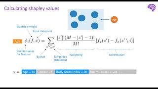
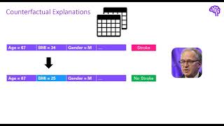
hi everyone in this video we will have a look at a popular explainable ai technique called shap the idea behind it comes from a different area which is cooperative game theory so give me one minute to explain you how it is used there imagine we have a group of different people that together cooperate in a game this group is also called a coalition and a cooperative game could be for instance a kaggle competition after the game is over they get a certain payout for their achieved results for instance they get ten thousand dollars for scoring first place now the central question here is how is that money distributed among the people so that the distribution is fair each member of the correlation contributed differently and therefore splitting it in same parts might be unfair for some the answer to this question is called shapley values introduced in 1951 by lloyd shapley shapley values tell us the average contribution of a player to the payout they fulfill a couple of nice properties and they are the solution yielding a fair distribution the explainable ai algorithm sharp makes use of these shaply values instead of using players in a game we can simply think of features in a machine learning algorithm each of these features contributed differently to a prediction so the prediction would be the payouts here and the game would be simply the machine learning model and that summarizes the basic idea we treat each feature like a player in a game and calculate sharply values to find out their contribution in the black box model the main intuition behind shapley values is that we want to compare how the correlation would perform with versus without a specific player this way we can find out how this person contributed in the game let's say for instance we remove this blue guy he has a strong domain knowledge about the problem addressed in the kaggle competition and without him the team would only place second instead of first the second place would be three thousand dollars instead of ten thousand so the contribution to the payout for this player would be seven thousand dollars however it's not as simple as that because we also need to consider the interactions between players let's say that the blue guy which is our domain expert only achieves great results if he works together with the orange guy who is for example an expert in deep learning that means that the contribution should be split among them to find out the true contribution of an individual player we also need to consider subsets of players for example if we consider this highlighted subset of our team removing the blue guy now doesn't lead to a big difference because the orange guy is missing anyways and that's why the basic idea of shapley values is to calculate a player's contribution for each subset and then simply averaging over all of these contributions this gives us the marginal contribution of a player to the team so that's also called the marginal value now let's move back to the machine learning context we said that we can for an individual prediction treat each feature value as a player and the payout as the model prediction sharply values tell us then how this prediction is fairly distributed among the individual inputs the explainable ai techniques sharp simply makes use of these sharply values shap stands for sharply additive explanations and is generally a local explanation technique so that means it aims to explain individual predictions of black box models however it is also possible to get valid global explanations through aggregating over these individual predictions let's have a look at the formula for sharply values and talk about how we can interpret it this expression gets us the sharply value for a feature i thinking of our previously used stroke data set for example we are interested in the contribution of the feature h and when i say feature i mean a specific feature value so for instance we have a value of 70 here as input for this calculation we have the black box model f as well as an input data point x this data point would be a single row in a tabular data set such as shown by this example now the first thing we do is iterate over all possible subsets set prime so combinations of features to make sure that we account for the interactions between our individual feature values the reason why our sampling space is denoted with x prime here is because for more complex inputs like images we of course don't treat each pixel as a feature but instead summarize them in some way using a mapping function we can then transform x to x prime but this is not really relevant in our example so one of those subsets could be for instance a subset of age and body mass index this means we only consider to have information for those two we don't know the values of gender and heart disease and the other features and now the most important step we get the black box model output for this subset with and without the feature we are interested in so in our example it's h the difference in those two tells us how h contributed to the prediction in the subset for example the black box model output with h would be seventy percent stroke and without age only ten percent that means h contributes sixty percent or with stroke in the subset that's also called the marginal value and then we do this for each possible combination so each permutation of subsets each of those is additionally weighted according to how many players are in that correlation or in other terms how many features of the total number of features are in the subset so capital m here is the total number of features let's say 20. the intuition is that the contribution of adding the feature h should be weighted more if already many features are included in that subset so that would tell us that this specific feature gives us a strong change in the prediction even if many other features are already included on the other hand we also want to give more weight to small correlations because there we have the features isolated and we can directly observe their effect on the predictions however there is one more question how do we exclude a feature from a machine learning model typically the inputs are fixed size and we cannot just remove parts of it because then the shape would change the way how this is solved in shape is that for the features we want to exclude we just input random values from the train data set if we do this for all subsets when calculating the contributions the relevance of these features is basically sampled out that means we completely shuffle those features and therefore make them random and as you might know a random feature has usually no predictive power let's talk about the complexity of calculating sharply values before we jump into the code calculating all those permutations so subsets is computationally expensive more precisely getting all possible subsets is an exponential term 2 to the power of n where n is the number of features for example if we have 10 features there are 1020 possible combinations for the subsets and therefore we need to perform a lot of calculations to get the average contribution of one single feature so here the blue ones stand for the features we want to include and the gray ones are the ones we basically want to remove in the subset the basic idea also presented in a chef paper is that we can simply approximate the shapley values instead of calculating all combinations kernel sharp for instance samples feature subsets and fits a linear regression model based on these samples the variables in this linear regression model are simply if a feature is present or absent so that would be blue and gray in our example and the output value is the prediction after the training the coefficients of the linear regression model can be interpreted as approximated sharply values this is quite similar to lime which we've seen in the last video however here we don't really care about the proximity and instead we weight our samples according to how much information they contain remember that we previously said that large correlations and small correlations tell us most about the contribution of features besides kernel shaft there exist other approximation techniques for sharply values for example tree shaft or a deep shaft which are used for tree-based models or deep neural networks respectively these techniques are not really model agnostic anymore but can use the model internals to boost the performance when calculating shabbly values i will not go further into detail for these to keep the video short if you're interested in details i can recommend the shep paper or the interpretable machine learning book as great references so now i think we are ready to have a look at some code examples so let's switch to vs code so as you can see i changed the color settings in vs code because some of the plots from sharp were not quite visible in the stark theme so now i hope it's better with this sprite layout in the first step we again import the data loader from our youtubes file just like in the other videos and additionally i use the plain sharp python library because i think that this library provides better visualization techniques than the other library so again we just import those things then we get the data uh one second okay again we have around 8000 train samples and 1 000 test samples because of over sampling and the black box model is again this random forest classifier we get an accuracy of 94 but remember our data set is quite imbalanced so this performance is not so good because our model tends to always predict no stroke and this is of course also reflected in the f1 score so if we move on we can now instantiate this tree explainer and we can use this tree shaft which i explained previously which achieves polynomial time complexity when calculating the chapter values so not exponential anymore and for tree based models like random forest which is a ensemble of decision trees we can use those models to speed up the calculation so as i previously mentioned shep is a local explainability technique but can also be extended to global explainability and that's why i select some individual instances in our test data set so in this example i go from the first data point to second that means i only get the first data point so if i run this that's the data points so these are the features h and gender and so on and now i calculate the sharply values with the sharp values function on our explainer object and then we get the sharply values for this single instance now let's further inspect how we can interpret them so what we get here is an array of size 2 and in the first block we get the shapley values for our first class so that would be class zero and in the second block we would get the sharply values for the second class so in a binary classification problem you would get two outputs here because we have stroke or no stroke so the contributions are then stored in these arrays because we have one value that's the single instance and then 21 values for the 21 features in our data sets okay sorry i had to do a little adjustment here regarding these indices so now what we can do is we can check what is the prediction of our model of course but more importantly we can use one of the great visualizations included in that package and one of them is for local predictions the force plots but it can also be used for globe predictions so what i want to do now is i want to explain this one instance i've selected above here and this plot then tells me the prediction is zero and reasons why that prediction was made is because the age is relatively low so for 43 we tend to predict no stroke instead of stroke and also the other values tended to shift the prediction towards no stroke and another thing you can see here is that we have a base value of 0.499 that value is calculated as the average model output and that totally makes sense because either we have one or zero as a prediction so in between of that we would have 0.5 okay we can of course do that for any instance we're interested in so here is another data points we get the shapley values again and then we use them to calculate okay here the h is 13 so we get a quite similar picture in this case but what we can also do is calculate the sharply values for several instances and then use that knowledge to get a overall plot so importance for each of our features and that looks like this so we see we have two classes zero and one and the contributions are the highest 4h the glucose level and body mass index and then we get those importances down the line so besides those visualization techniques there are many others in chap here are some examples on the github project those waterfall plots also provide a nice way to see which feature value contributed most like here we have specific values so that's for local explanations the same here but we can also do it for a set of data points like it is done here and as you can see this library provides many ways to visualize the shapley values so the example we've seen was based on tabular data however shap can also be applied on other data types here is an example for a transformer model that means for a text data input or here is another example from the github project where sharp is applied on image input so i can recommend to check out the github page there are also many notebooks linked if you're interested in further details so that's it for the third video in the next session we will have a look at counterfactual explanations and as always the code is available on github leave a comment if you have questions and i see you in the next video