Logistic Regression - VISUALIZED!
Key Takeaways
The video explains logistic regression, a fundamental concept in machine learning, using visualization and mathematical concepts such as sigmoid functions and decision boundaries. It covers the training process, including optimization techniques like gradient descent, and demonstrates how logistic regression works for binary classification in one and two dimensions.
Full Transcript
on this channel I've made videos explaining some intuition behind logistic regression digging into the math now we cover topics like the sigmoid function linear decision boundaries and so much more but I want to get a more visual take on this and when we say we are training a logistic regression model what exactly is going on that's what we're gonna look in today so sit tight logistic regression as you may know is typically used for classification in machine learning did this passenger survive on the Titanic or not will this person defaults on their credit card or not in each of these cases we have a binary outcome and typically in machine learning we model such outputs as a probability so instead of having our model predict one the person defaults or zero the person doesn't default we instead have it spit out something like this person has a 60% chance of defaulting because of this such classification models have a fixed range of outputs to spit out between 0% and 100% we basically need a function that takes in any real number from negative numbers to positive numbers and squishes it into a probability logistic regression specifically uses a function called the sigmoid to do this squish off' occation fair warning the implications of using sigmoid can get fairly technical and I'd be happy to make a separate video for it however it for this video let's keep it simple and stick with the intuition that we use sigmoid because we want to squish any value into a probability ranging from 0 to 1 so the sigmoid function what does that look like let's start by first drawing a number line with two coordinate axis the x-axis will represent independent data points and y-axis will represent the values of our sigmoid function a simple sigmoid function would look something like this S curve and no matter what value X may take the sigmoid always has a value between 0 & 1 this fact remains true for any such sigmoid curve the y-coordinate always ranges from zero to one so this verifies that we can use a sigmoid function to model probability for example this point could represent the conditional probability that Y belongs to a positive class given a value of x I'd be remiss if I didn't give a shout-out to Grant's Anderson aka three blue one Brown the animations in this video were created using his math animation engine manum and I'll leave a link to it down below so check it out we now have a function that spits out a probability great but in the end we want a binary output that is a yes the person will default or no the person won't default now how do we do this from probability values we assign this using a threshold let's take it as a standard 50% here that is if the sigmoid function for a given value of X is greater than 0.5 it should classify the point as 1 and if it is less than 0.5 it should classify the point is 0 but note how you assign the threshold depends on the application in cases where we want less false positives a higher threshold is good in other cases where we want a higher recall a slightly lower threshold is good it's up to the developer to choose this threshold now question how do decision boundaries fit in for those not familiar with the decision boundary it is basically a boundary that the model uses to make decisions simple enough every point that falls on one side of the boundary is categorized as 1 and points that lie on the other side of the boundary are categorized as 0 unspeaking for the binary classification case but this definition can be expanded to multiple classes in multiple dimensions what you see here is a two-dimensional plane with axis variables X 1 and X 2 in a 2/2 no plane we have a two dimensional decision boundary in the form of a line or a polyline if we look at the one dimensional case with a single axis X we have a point decision boundary every point on one side is classified as 0 and every point on the other side of this boundary is classified as 1 now for multi-class classification we could use multiple points as the decision boundary now that we visualize decision boundaries how exactly are they created restated in another way given a set of these data points how does logistic regression know where to put the decision boundaries that work best well let's start with the one-dimensional case we mentioned how a function called the sigmoid function is used for determining probability in this one-dimensional case the function looks like this we've been here and done that it squishes a linear and put into a range between 0 and 1 in the context of logistic regression training we could also write this equation just replacing the X with B plus WX b is an intercept bias term W is the weight of the independent variable X on some response variable Y if we give a threshold of 50% then this final value is basically 0.5 let's simplify this to get an equation take logs on both sides and then we get this final form B plus WX is equal to 0 or this corresponds to a point X is equal to negative B by W but what does this represent this is the point decision boundary in the one-dimensional case for binary classification it is this point that splits your one-dimensional data points into two parts if you don't quite understand pause and think about how this is the case when the value of X is at the value negative B by W there is a 50% chance that Y is equal - one for binary classification problems also if X were greater than this value the probability of Y being one would be greater than 50% and if X is less than negative B over W then the probability of Y being one would be less than 50% I hope you understand this great so now we know the equation of a point decision boundary it's X is equal to negative B over W but we don't have W or B but we can find this out through the training phase of logistic regression what does it mean to train a logistic regression classifier it means finding W and B that maximizes the probability of seeing the training data I made a gentle explainer video on logistic regression and a maximum likelihood estimation before so I won't get into the math details right here my objective is to visualize logistic regression and training during training we can use a step by step technique of changing W and B until they've reached their optimal values and this is done with optimization techniques such as gradient descent it is a technique that involves changing the values of W and B ever-so-slightly to maximize the probability of seeing the training data I'll get into the details mathematically in my next video but know that the update equations for the weights and the bias looks something like this we start by initializing W and B to some random values or just one in this case for some M iterations we change the parameters ever so slightly that W and B will converge to their optimal values W sub M and B sub M here alpha is the learning rate aka how fast do you want to learn n is the number of training samples X I and y i are the eighth training sample X is the features and Y is the binary label and Sigma is the sigmoid function don't worry if you don't understand this completely but let's visualize what this math is doing maybe you'll get a clearer picture let's consider the one-dimensional logistic regression case for a binary classification we have some training sample points they are labeled as 0 or 1 by color here let us just take the initial value of W and B to be 1 each like we stated before I'll set the learning rate to be a typical value like zero point zero five zero point zero one whatever it is depending on your data from this we can determine the initial decision boundary X is equal to negative B over W which in this case is negative one and now we're going to start the training phase we apply the update rules for W and B and because of this update the decision boundary changes continue to the second iteration and now the third iteration and if we keep applying this for some time we eventually see W and B converge so basically the decision boundary stops changing it by much eventually I'll play this entire training process again but this time let's also visualize how the sigmoid function changes at every iteration you for every point X the height of the curve above that point represents the probability of that point belonging to the positive class that is y is equal to 1 pretty slick right now during the testing phase when we are passed some data point and our models asked to label it we first determine the probability that this point belongs to the positive class and then assign its class depending on the probability so what we did until now was visualize two major concepts the sigmoid function and the decision boundary but both of these are just for the one-dimensional logistic regression case let us visualize how these change for two dimensions when we have two features we have the original sigmoid function here for the one-dimensional case the sigmoid function squishes the linear input of one variable X into the range 0 to 1 so we have this curve but now we have two features x1 and x2 the sigmoid should now squish a linear function of features x1 and x2 into the range 0 to 1 so we have a surface with this equation B is again the bias term w1 is the weight of the independent variable x1 on some response variable Y and w2 is the weight of x2 on the same binary response variable Y if we give a threshold of 50% then this entire value becomes 0.5 let's simplify this to get an equation in the same way we did for the one-dimensional case take logarithms on both sides and we get the final form B plus w1 x1 plus w2 x2 is equal to 0 now this equation corresponds to the equation of a line with X 1 and X 2 as the two axes so this is also the lying decision boundary in the two-dimensional case for binary classification it is this line that splits your two dimensional data points into two parts once again if you don't quite understand this pause and think about how this is the case for a data point x1 x2 when the value of the equation is zero there is a 50% chance that Y is equal to 1 for the binary classification problem also if this equation is greater than 0 the probability of Y being 1 would be greater than 50% if the equation was less than 0 then the probability of y equals to 1 would be less than 50% to find this line we need to know the coefficients B 1 W 1 and W 2 and this is done during the training phase of logistic regression using the same gradient descent algorithm so here was the algorithm for the one dimensional case and now here's the update for the 2-dimensional case the only difference that I made is now making W and X bold this is just simple math notation to show that these are vectors in the two dimensional case they are vectors of two dimensions for a clear picture like we did for a one-dimensional case let's visualize how this two dimensional line decision boundary is created back to our black screen consider a 2d plane with axis x1 and x2 we have some training sample points that are scattered in some way in this plane remember for each point we have a label indicated by colors let's take the initial values of the weights and bias to be one each I'll set the learning rate to be some fixed value from this we can determine the initial decision boundary B plus x1 plus x2 is equal to 0 to start the training phase we apply the update rules for the weights and bias to get that slight shift in values now the second iteration of gradient descent now the third and if we apply this for some time we eventually see the weights and bias converge you and look what we have here we have a decision boundary in the form of a line and guess what this line has the equation of the form B plus w1 x1 plus w2 x2 is equal to 0 now where does the sigmoid fit in I'll play this entire training process again and this time let's also visualize how the 2d sigmoid function changes at every iteration you for every point in the x1 x2 plane the height of the sigmoid function would represent the probability of being in the positive class that is y is equal to 1 so during the test time when you are given a point x1 x2 you first determine the probability value and then assign the predicted class based on that probability value of it being either the positive class or the negative class great we visualize the sigmoid curve and the creation of a decision boundary with logistic regression for the one and two dimensional cases but this begs the question how do we go beyond this how can we think of multiple dimensions greater than two now I can't create visuals for this myself because I can't effectively demonstrate four-dimensional plotting on screen but we can easily expand our intuition on this for the one-dimensional case we have this and for the two-dimensional case we have this expanded equation with w1 x1 and w2 x2 but we can also rewrite this in vector notation treating W 1 and W 2 as a W vector and also X 1 and X 2 as an X vector now for some arbitrary M dimensions we can write the same equation form but X and W instead of being vectors of two dimensions they are now vectors of M dimensions and that's the only difference here we can use the same argument for every process gradient descent for one dimension we have the update equations that look like this in the two-dimensional case we introduced W and X as being bold as they are now vectors of two dimensions and for the higher dimensional gradient descent all the equations are the same all we do is replace the two with the order of dimensions and that's it I hope this video helps you visualize logistic regression training in one in two dimensions and gave you an intuition on how you can think of higher order dimensions no there is a lot more to logistic regression and I'm going to be deriving all these equations from scratch in my next video so that's gonna be fun some learning resources are down below but stay subscribed and I will see you in the next one buh-bye
Original Description
People talk about "sigmoid functions", "decision boundaries" and “Training”. But what exactly is happening behind the scenes? Let’s see for ourselves!
Please SUBSCRIBE to me for more content!
Shoutout to 3blue1brown for creating his animation math engine “manim”. Give this a * on your way out: https://github.com/3b1b/manim
REFERENCES
[1] My previous video on Details of logistic regression (I’ll make another one soon): https://www.youtube.com/watch?v=YMJtsYIp4kg
[2] More on Generalized Linear Models: https://www.sagepub.com/sites/default/files/upm-binaries/21121_Chapter_15.pdf
[3] Logistic Regression & GLM: https://newonlinecourses.science.psu.edu/stat504/node/216/
[4] Overfitting problems in Logistic Regression: https://courses.cs.washington.edu/courses/cse446/17wi/slides/logisticregression-overfitting-SGD.pdf
[5] More info: http://byrneslab.net/classes/biol607/lectures/lecture_19_handout.pdf
Watch on YouTube ↗
(saves to browser)
Sign in to unlock AI tutor explanation · ⚡30
Playlist
Uploads from CodeEmporium · CodeEmporium · 35 of 60
1
 2
2
 3
3
 4
4
 5
5
 6
6
 7
7
 8
8
 9
9
 10
10
 11
11
 12
12
 13
13
 14
14
 15
15
 16
16
 17
17
 18
18
 19
19
 20
20
 21
21
 22
22
 23
23
 24
24
 25
25
 26
26
 27
27
 28
28
 29
29
 30
30
 31
31
 32
32
 33
33
 34
34
 ▶
▶
 36
36
 37
37
 38
38
 39
39
 40
40
 41
41
 42
42
 43
43
 44
44
 45
45
 46
46
 47
47
 48
48
 49
49
 50
50
 51
51
 52
52
 53
53
 54
54
 55
55
 56
56
 57
57
 58
58
 59
59
 60
60

Linear Regression and Multiple Regression
CodeEmporium
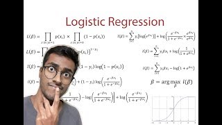
Logistic Regression - THE MATH YOU SHOULD KNOW!
CodeEmporium
Generative Adversarial Networks - FUTURISTIC & FUN AI !
CodeEmporium
Deep Learning on the Cloud - GPU TO LEARN FASTER
CodeEmporium
Deep Mind's AlphaGo Zero - EXPLAINED
CodeEmporium
Mask Region based Convolution Neural Networks - EXPLAINED!
CodeEmporium
Attention in Neural Networks
CodeEmporium
Depthwise Separable Convolution - A FASTER CONVOLUTION!
CodeEmporium
One Neural network learns EVERYTHING ?!
CodeEmporium
Neural Voice Cloning
CodeEmporium
AI creates Image Classifiers…by DRAWING?
CodeEmporium
Unpaired Image-Image Translation using CycleGANs
CodeEmporium
K-Means Clustering - EXPLAINED!
CodeEmporium
Random Forest Classification
CodeEmporium
Data Science in Finance
CodeEmporium
Hypothesis testing with Applications in Data Science
CodeEmporium
A/B Testing - Simply Explained
CodeEmporium
The Kernel Trick - THE MATH YOU SHOULD KNOW!
CodeEmporium
Support Vector Machines - THE MATH YOU SHOULD KNOW
CodeEmporium
Principal Component Analysis (PCA) - THE MATH YOU SHOULD KNOW!
CodeEmporium
History of Calculus - Animated
CodeEmporium
Curiosity in AI
CodeEmporium
DropBlock - A BETTER DROPOUT for Neural Networks
CodeEmporium
Autoencoders - EXPLAINED
CodeEmporium
Recurrent Neural Networks - EXPLAINED!
CodeEmporium
LSTM Networks - EXPLAINED!
CodeEmporium
Building an Image Captioner with Neural Networks
CodeEmporium
10 Machine Learning Questions - ANSWERED!
CodeEmporium
How do neural networks work?
CodeEmporium
Evolution of Face Generation | Evolution of GANs
CodeEmporium
How does Google Translate's AI work?
CodeEmporium
How to keep up with AI research?
CodeEmporium
How does YouTube recommend videos? - AI EXPLAINED!
CodeEmporium
Variational Autoencoders - EXPLAINED!
CodeEmporium
Logistic Regression - VISUALIZED!
CodeEmporium
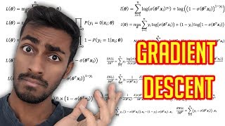
Gradient Descent - THE MATH YOU SHOULD KNOW
CodeEmporium
Boosting - EXPLAINED!
CodeEmporium
Transformer Neural Networks - EXPLAINED! (Attention is all you need)
CodeEmporium
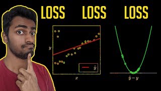
Loss Functions - EXPLAINED!
CodeEmporium
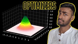
Optimizers - EXPLAINED!
CodeEmporium
NLP with Neural Networks & Transformers
CodeEmporium
Batch Normalization - EXPLAINED!
CodeEmporium
Activation Functions - EXPLAINED!
CodeEmporium
Data Scientist Answers Interview Questions
CodeEmporium
Why use GPU with Neural Networks?
CodeEmporium
How do GPUs speed up Neural Network training?
CodeEmporium
BERT Neural Network - EXPLAINED!
CodeEmporium
ConvNets Scaled Efficiently
CodeEmporium
Transformer Neural Net makes music! (JukeboxAI)
CodeEmporium
What do filters of Convolution Neural Network learn?
CodeEmporium
We're hosting a Machine Learning Conference!
CodeEmporium
MLconfEU 2020: Machine Learning Conference for Software Engineers
CodeEmporium
Are Neural Networks Intelligent?
CodeEmporium
Time Series Forecasting with Machine Learning
CodeEmporium
Few Shot Learning - EXPLAINED!
CodeEmporium
How does a Data Scientist Fight FRAUD?
CodeEmporium
How would a Data Scientist analyze Customer Churn?
CodeEmporium
Expectations with Machine Learning
CodeEmporium
Why Logistic Regression DOESN'T return probabilities?!
CodeEmporium
How you SHOULD code Machine Learning
CodeEmporium
More on: Supervised Learning
View skill →


Related AI Lessons
⚡
⚡
⚡
⚡
Mastering TypeScript — Understanding the TypeScript Compiler (tsc) from Scratch — Lesson 2
Medium · JavaScript
Stop Overfitting With Basically One Line of Code
Medium · AI
Stop Overfitting With Basically One Line of Code
Medium · Machine Learning
Stop Overfitting With Basically One Line of Code
Medium · Data Science
🎓
Tutor Explanation