Dive into Deep Learning (Study Group): Modern CNNs | Session 7
Key Takeaways
The video discusses modern CNN architectures, including AlexNet and VGG, and their applications in computer vision, with a focus on convolutional and pooling layers, feature extraction, and network design.
Full Transcript
okay so good morning everyone it's 601 maybe we'll wait um couple more minutes so and again uh today's session after today's session so we covered the fundamentals of CNN last time uh there was enough to now go over any CNN and um understand it and that's what we will do today so we're going to cover a few and we'll also do the the Hands-On coding of them and if there are new ones which they come out all the time you should be you should be comfortable enough to understand any architecture so that's the goal so maybe we'll just wait a minute or two and then we can get started uh so again where we left off we uh we pretty much we did Lunette last time and again we're just following so again how this is a study group right so like we're just uh following the Deep dive into uh dive into deep learning so I'm also trying to follow that that format so like now after learning we're going to go through alexnet and so forth until reset and denet and so forth okay so I guess we can go ahead and get started and we will do a small recap in the beginning and we'll do um few Recaps all the way through okay so um okay let's just recap what we talked about uh I have another recap slide but let's just um Talk about uh computer vision and cnns uh before um computer vision before before even CNN what we talked about was computer vision was really more about feature engineering so for example even if you wanted to do like Edge detection like so for example now after what we saw last time we give an example of how we can use uh CNN to detect edges but back um back all that was actually manually done so and again we saw how like Lunette was in the '90s but then it kind of it fell out like there was no no hype going on nothing came out like on the early 2000s for a few reasons that we're going to talk about primarily the data sets Wen there the right data sets and hardware and then they came back after primarily with imet Okay so let's get started so this first slide uh we saw it already right and then pretty much here uh so this is kind of like the end so I just picked up like the last kind of slide and then uh we'll go into depth so pretty much this is um the mest data set that we applied our lunet on and then what we talked about uh what are these These are feature Maps so these they would extract like the what we call them the low level features like maybe edges and so forth and then and so forth and then until we get our here until we get we classify and then we say for example here which number is it from the 10 numbers for example mest right we're classifying from 0 to9 so um so every after every con layer we extract features and to to get to um to our final results okay so uh then what I wanted to share is um there is by the way um there is a nice paper let me just take that there is a nice paper where uh I took this visualization from and what they did they tried to visualize the features that they we're getting throughout the layers and um you see how we talked on the last slide about the edges so it's kind of like same thing so you can think of it that on the first layers we extract edges colors and so forth and then on the following layers it's more complex structures like you see here and here what they try to do they just try to kind of like match oh they said oh okay these features they match these kind of images and so forth and then on the much higher levels then we we extract like the feature Maps is just like an aggregation of different features together okay so um okay so now let's get into it so we talked about uh computer vision was more feature engineering you see like how right now what we did we were we were feeding pixels directly into our Network so was never the case like people would never kind of like feed just raw pixels into their into their networks they would they would they would process them a little bit they would try to get something from them just like if you're doing traditional machine learning and then from that then they would just feed it into something for example back then svms support VOR machines were the ones that were working very well until uh until convolutional layer convenant kind of like um around 2012 this when but yeah so so so the Breakthrough was uh because of two things primarily the data sets and okay so let's talk about the data sets it's not like there wasn't data sets back then there was this very popular actually um uh repo that's still there right now it's called called UCI it's I believe from um I believe maybe it's Berkeley or but if you just Google UCI dat sets it's a good actually it's a good collection of many data sets that um uh they range from from Health Care to to just random images and so forth so there were those but the quality of images wasn't great and there were um it's and so it's there weren't the best images so the data sets overall weren't the best so that's one thing primarily datet and that's when imag net came so imag net came from Sanford so they said you know what why not let why not make this big data sets and then challenge all these researchers whoever going to classify this thousand for example this this thousand classes right and so forth and and so they scraped images from the web and then they used this Mechanical Turk of Amazon where you pay uh people to to annotate images for you and so there was a lot of effort from uh from the staff at Stanford to actually put this together but it's something that really drove there something that was the Breakthrough that's something that drove the whole field and the community so um so that was great so that was in 2010 so uh there was in well the data set was was released in 2009 but really the challenge when they challenge it started in 2010 and still uh 2011 and you're going to see this 2011 and 2012 it the winners were not based still on convolutional Nur Network they were still based on just shallow what we call them just shallow um uh computer vision models and then Hardware Hardware second point and I'm going to ask you throughout this why and then I'm I'm going to ask you the question now and then maybe you can think of it and then we'll we'll see we'll talk about why later but why I mean we saw it kind of in a way why do we really need a lot of compute with deep learning and and I and I want you to have this clear this is why and this is why and if I say okay can you show me an example you be like okay here is an example and this is why and this is why deep learning you really need a lot of computes so so that's another thing um that's another thing so for example we saw we saw nness right we were just seeing a 28 by 28 resolution images but I mean again computer vision we're talking about how about high resolution so like now when we talk about like a much much higher resolution images and big data sets to process all that you definitely need a lot of comput and we'll we'll do some some fun math today with that okay so I think that's good so now before getting into the different architecture so again I'm going to I'm going to say again the goal of today uh a successful session would be by you after this session whatever one hour and a half two hours you're going to leave that you are comfortable at digesting any CNN that you will look at that you will that you will find online either uh you know something that that was there we didn't cover or something that just going to come out okay so that's the goal and how we're going to do that we're going to do that by covering different ones and you're going to see oh okay this is pretty much the pattern this is pretty much how one Builds on top of the other one and then actually not only that it's going to give it's going to give us a way of how researchers even think of ways to improve thing to improve the the networks things changed lately like back in the day you can get like a paper published by Just For example just changing some we pooling okay let's talk about this pooling and strides and all back then you could you could actually get a nice paper published by just uh playing with this hyper parameter let's say you know playing with the hyper parameters and just uh doing some tweaks here and there and then and then with the data set you can get some good results and you can get your paper published now maybe it's a little different because uh but yeah Okay cool so um so what do we have here okay so let's go let's go let's go over this so now when we see this we all know what we see in this um in this network or this architecture we have an input image and then um we apply convolutional to it and then we talked about kernels we talked about filter [Music] um we uh okay we talked about channels in channels out okay um so we talked about the output shape size so for example if you are given okay so and here's a question now that I'm asking you and then we're going to go through it but if I'm giving you an image here and I will tell you hey this image is 20 um 20 8 by 28 or 100 by 100 okay let's say this image is 100 by 100 and I'm giving you a 3X3 kernel okay that's that's the size of your kernel is 3x3 and maybe you do pad in size of one what does again pad in size of one here we see it here meaning what meaning we P to the left we pad to the right right and we and and we pad up and down and then if I say okay you have that and you're doing a stride of two what is your what are you expecting as your output what's the side so you'd be able to do that okay so that's something that we saw and then we have other features and so forth and then we call this feature Maps Okay so we call this future Maps so this is this is now what we've seen very common so we said we're going to take a picture we're going to do some con layers here and then at the end we're going to feed this to fully connected layers and then here we just do some soft Max and then we get our um uh so for example here a multi cross entropy so so we get which class is it from all the different classes okay uh if it's uh if it's a binary classification it's just two classes if it's many classifications okay so that that's what we seen and here what we seen is the p padding um we talked about stride is by is how much do we move so we talked about padding how much do we pad and again why do we why do we again pad because if we don't pad we Som how like really the output would just shrink so fast right so that's the reason for padding strides is like the other way it's like actually when we in purpose when we want to like really shrink the image uh going down and then what else did we so we saw pooling right and then with Lunette um it had average pooling right but we still but we still because Max poolin wasn't really um applied back then or they didn't think of it back then but we covered both we said this is what's Max pooling is and this is what average pooling is and um I believe we covered a few other things but these are the core things that we're going to uh use from today from that that's going to be helpful for today's session Okay cool so so far I I I believe we're all in the same page okay so what we're going to cover today so um as as I said so okay it was released 2009 or the challenge was in 2010 uh so these first two ones were not based on confet so what we're going to cover today is the first winner of the challenge alexnet uh all the way through until reset actually all the way through even we may discuss even what comes after resonet there is even there is another session uh I believe uh it's chapter 13 or so that we're going to that we're going to do together and um and we can even go more advanced in that but after covering all this all of us should be fine actually Digest again any uh convolutional Nur Network okay so that's the plan so we're going to cover that we're going to do we're going to code it we're going to um this one okay we'll see that and we'll see all of them okay so um and this is and so what I tried to also do uh yes uh we are definitely following the format of of the book so that way even if I miss something or if you're confused about something I don't mention it you can just go back and read it again it's a book that I personally like it's one of my favorite books of of deep learning uh but I tried to show different images and diagrams of cnns because everyone you'll find different papers you're presenting it differently you know and so forth so I would present here for example to the right or to the left how the book have it but I would also present a different format so that way however you see it you you you know exactly what's going on okay so for example the book they just show alexnet like this we should still be fine to know exactly what what what's what's happening here based on what we did before for example we say oh okay the image input size is 224 by 224 what three oh okay three channels okay what do we do next we do a convolutional of Kernel size 11 by 11 oh what's 96 oh 96 is our output channels oh we have a stride of four and so forth Max pooling oh already covered Max pooling what's uh the max pooling right there are no parameters to be learned there but there is the window size so this Max pooling is a 3X3 this Max pooling has a stride of two meaning what meaning it moves to kind moves two strides at a time and so forth and then so we have 11 by 11 kernel and then the next conve layer would be 5x5 then the next we do some again same one and then the next conve layer would be 3x3 and so forth what has changed so small things Has Changed For example we can see that pad in here they padded throughout the way differently so for example here you can see that they padded here by two and then after that they padded here by one and then uh stride here four then here okay uh well this stri is for con layer this St to is for the max pooling okay uh but but then you may be asking so so based on what based on what are they really changing this and that is a valid question to ask and we'll see and we'll see and we'll see the answer of that later okay so good and then again the format how was the the format or the structure of this the structure of this um uh networks that we saw we had con layers so far what did we see so far we we saw only Lunette Lunette had con layers and then it was followed by fully connected layers and these I Believe by now after after you have uh went through the MLP chapter and all you're all masters of this of this one okay the fully connected connected one here there is there is nothing much going on here on the fully connected they're just all as the name says it's fully connected okay but what's different is here there is a step between here and here which again on when we code we call it like we flatten we flatten our 2D uh to be 1D and then we change here for example we just kept side the same size and then here we change it to one to 1,000 why here for example 1,000 because because again this was for the image net challenge the image net challenge they were trying to predict thousand different classes okay perfect so so now now we know that but let's see you will see different uh uh structure so for example now you're going to see something like this uh just in maybe in less than a minute uh this should also uh we go over it and it should also make sense so for example what do we have here we have the size okay 227 by 227 we have the kernal 11 by 11 okay we have three which is representing here the depth the number of channels three okay now uh here we we apply our con layer uh which is again you see that con layer of k 11 by 11 each here and then we have D stde would we get uh we get 55 by 55 and then here we have a depth of 96 so now I'll ask you where did this 96 come from so this 96 for it to be here that means actually our kernel had to have 96 filters within it I mean it it had to have well the filters actually the filters of the C layers have to um to be the same as the input channels so actually for example um and that's the thing sometimes so so don't be confused with kernels and filters so because even myself sometime I use them uh interchangeably but it's fine so but here's what here is what we have to to understand uh every kernel we have an inut we have an input say for example three for example here we have RGB three channels for for that kernel it has to have three we can call them three different um we can call them three different kernels so we can actually multiply that by the by the the the channels okay but now let's say if we want to have many channels out so we want to have now many channels out so we're can to have one and for example here we're going to have 96 right so now meaning what meaning we're going to have 96 of those kernels 96 of those kernels which each kernel have three okay so we have 96 and each of those 96 have to have three um here's what I'm going to call them I'm going to call them I think this is how I called them last time too 96 uh filters and every filter has three kernels okay because now the input I believe that that's clear okay and that's how this 96 came came about and and so forth and then we keep going so forth for example here Max pool in 3x3 window a stride by two um that's again Max pooling if if you get asked about what is pooling pooling is just the same as down sampling that's pretty much either you do average pooling or you are doing Max pooling you are really just down sampling the size of your of your of your input whatever input image your input feature map right we call that we call these feature Maps right um again so feature Maps because yes you can think of these as feature as features what they have inside sometimes they're also called elements that's also fine okay okay okay so that that's all that there is so now we can see how this is really if you see something like this this is just same as if represented like this so we have a con layer here and then we have a a Max pulling layer here we have a con layer a Max pooling and so forth and so forth uh until we get here and then what we do here we have a 6x6 and a depth of 256 okay and then we flatten that out to get this 4,000 and 96 and then we have another fully connected layer and then we just apply soft Max okay um so so and and I'm gonna pause for a second please type your questions and Elvis uh he he will he will ask me the questions and I will pause here and there but let's do maybe this this couple problems uh and then I'm going to pause right after them so this is also a recap but we're all so here what I want to do I want to do a recap from what we've seen before but we're applying it to to actually by the way do you see any inconsistency here is there something on this slide um which is oh you know so if you may see like and this is taken from the book it's 200 by 20 200 uh 224 by 224 but here 227 uh 200 27 by 227 so which one is the right input image so um so how about then if I tell you you can you can tell me you know you can tell me which one okay how how can if I tell you hey how about for this assuming that this is the correct output size this 50 55 is the correct output now just go back backwards which one is it okay so so so just do that and you will know and and actually you can go online and so the paper actually the the Alex paper this is exactly what they had they had 224 uh but there were things brought up about this 227 some said that the paper did not have the correct input size but now I can let you figure that out okay okay so um so let's do let's do a problem now um and we're only going to now do this calculation for one layer for one con layer and if we are able to do this for one conve layer we can do this for any any conve layer no matter the stride no matter the pattern no no matter what the kernel size is okay so again we're going to go with the 227 here okay and then we have three channels because it's RGB and then we say we have 64 filters and our kernel size is 11 by 11 okay so I'm going to pause again here I'm just going to repeat what I just said a second ago we have 64 filters and our kernel size is 11 by 11 okay that means for us for us to do to be able to multiply to do our convolutional uh convolution we have have to have three of these kernels we have to have three of them so that way we can multiply them with our channels in okay good and how many times we're going to do that we're going to do that 64 all the 64 filters and then we have our stride four and our pent two if if I were to ask you what is your expected channel number of your channels out okay you're going to say oh this is easy you have 64 filter is 64 okay that's correct 64 how about the output size of your um height and width how can you actually get that the output now size of your expected feature map height and width that's when remember this equation that we saw okay you remember this I think we saw it at the very end we take this this is our size input size plus 2 * padn minus the size of the kernel so for example here it would be 64 plus 4 so 68 - 11 so 57 over 4 + 1 anyways I hope I did that correct but that's how we we we get it okay um uh so input size so what's the input size here what's the input size it's the is 200 2 27 so if you do 227 plus that 227 plus uh 4 which is coming from the pad minus K the 11 C over stride plus one you should get 56 okay good now that we so this is just a recap um if I were to ask you okay so now we have this we have this um I don't know if you are looking at my face but sometime I just you don't have to if it's distracting for you don't but sometimes I just uh I just move with my with my finger so let's say for example we have this feuture map right and this feature map now I have this size of 56 56 and there are 64 64 output channels if I were to ask you what's the memory how much memory do we need to store this uh so that's something that we not cover but it's something uh good to know good to know because all the networks that we're going to see today what they tried some of them what they try to do they try to be of course efficient efficient in the compute and that's how they come up with different architectures so it is good to know how much memory is this taken okay so let's see that so um so how much memory is this output for us how much memory do we need to store this output okay our output is 56 by 56 so we have to multiply that time 64 that's all okay so that's the number of elements you remember I said elements or features call them whatever you like because it's a feature map that has features you can call the elements that's also correct so we have 200,000 of them let's assume that we are working with a 32bit floating Point okay so a 32 bit floating Point meaning to store one element to store one element we need 32 bit right and maybe this is just go to um to our basics of just bit and bite one BTE is eight bits so for example for 32 bits we just need four bytes okay so we need four bytes to store one element meaning here we need four bytes times the 200 that's how many bytes we need if I and then if I and if we're asked how many kilobytes then we just divide by 10 to the power three this is the same if you divide by TH or uh or ,24 this 1024 is just coming from uh from two to the power uh two the power uh8 or 10 to the power um uh anyways you you do the but anyways the right one is ,24 but is th000 so that gives us um because this is this is actually in in in memory and compute this is how it is so this is actually the right one but you know usually we just say when we say kilobytes is just thousand say gigabytes you know it's just 10 to the^ three 10^ six and so forth um so okay so this is how how much memory we need to store that uh now if you're asked how many parameters and this is also very important uh you know how how last time we talked about different convolutions and which one maybe you want to use maybe you get to a point you say you know what I'm I'm I'm planning on on using on using all this for um for Edge devices so you definitely want to want to know how many parameters so for example how many parameters here um uh is it's just the calculation that we mentioned earlier so we just we have that kernel 11 by 11 we have three channels but we need to do that for all the 64 filters right so that's the number of Weights that we are learning right hyperparameters parameters so these These are the the weights that we are learning where does these weights they are where do they go they go inside our kernels and if you want to visualize them they go inside the kernels perfect so that's the weights and we have weights and biases right every filter would have one bias so now we'll just add this to that and these are our learnable parameters for only this specific con layer one perfect so now this is what we know this is our two uh 23,000 is our un learnable parameters um okay uh this is the last one this is the last question but uh so so now because what we're trying to get to we're trying to get to how much compute right and um so how many operations then how many okay so now so now we know uh the memory here what did we say the memory to store our output side output right the output from the comp layer good that's our memory to store that the number of parameters that we need to learn so how much operations did we do did we just do in that one kind of layer I mean again we just did the 11 by 11 times that three uh because we had three input channels right and we had to do that for 64 filters so just same one but we had to do that to fill in every feature right we had to do that to fill in every feature of our output size this must be our output size you see how it is 56 so all this those are the number of operations uh here here we are you may be wondering where's the bias yes uh we actually we certainly can add the bias here but then then where would you add the bias actually uh you would add the bias right here so it's going to be 11 time 11 * 3 plus one plus one of the bias times all that but you know one is it's not much you know it's just going to increase this by a bit but here you see where we get 72 million okay so 72 million operations okay so I'm going to pause it so 72 million operations and this is sometimes when uh so that's for one C layer one C layer for example here it has 23 23,000 parameters and it had and it's doing 72 million operations um and this is okay and you often hear you know when we talk about gpus and all that we often talk about flops uh and flops are exactly this the float and point operations per second this GPU that you're trying to buy how many float and point operations per second can it do you know like so for example is um you know I don't know how much background everyone is coming from so I'm just sharing this and and and ex excuse me if this is uh if this is just uh you know just uh basic basic stuff but you know there is like for example CPU for the clock cycle we say how many Herz for for gpus we say how many flops and it is for example it is a measure of the compute performance okay okay next so so okay perfect so now we did all that now uh okay this table is filled out for you now I want you to notice something I want you to take a second and look at this table look at especially here the things that we calculated and try to notice something especially from okay the H if if we are comparing the con layers with the fully connected layers can you can you compare like what do you see there you you what we see is we see that the con layers they have a lot more parameters right because they're fully connected a lot more parameters but they don't really have a lot of operations and that is very important to understand that while even if the coners they have less parameters they're very heavy in computation okay and and then something okay perfect and this is the only thing that I wanted to mention uh moving forward because we just want to remember this throughout our work because again for us to to have fast training and all that this is what matters we want we want to have the least number of operation but still getting the best accuracy the best performance metric whatever performance metric you're you're going for okay good so um the last thing before I pause I want to I want to share here um and these are things that weren't necessarily shared on the book but I feel like these just kind of extra things just they help solidify everything put everything together um so good so Alex net uh Alex net had many U had many things that that for example we saw um we saw how it had more con layers than lunet that's that's for example one and um uh it had what what else I mean we can go back and for example here we can just see if we if you remember laret leet um so for example here they used 11 by 11 a much bigger kernel size than before but why why did they use this much bigger kernel size because of course here the the images are bigger right than before Emin they were dealing with only 28 by 28 so here they needed to so and one of the things that um alexnet introduced that was significant is the way how how ilas and Alex they they implemented it so they realized exactly what we just seen and they realized they said heyy you know there are 62 million parameters okay and there is one billion computation right and they found out that most of the parameters are coming from from where most of the parameters are coming from the fully connected from the ful connected uh layers but most of the computation is coming from where it's coming from the convolutional layers and this was actually their motive of they split it into this two um Invidia Nvidia GeForce uh gpus back then only three gigs of vram but it definitely it was it it was it was a good a very good um iteration and breakthrough okay and that that's other papers build upon um okay so um so and and here by the way here so based on that based on the on this they they publish another paper that you can check out that that I have the link here for okay uh but this is how it was implemented and if you want to even look into the details you will see that how all of these they were and again a different maybe structure that we did not see before but you see it you understand it there is nothing here that you say oh okay it's just the input 11 by 11 kernels oh okay you just said that they split it into two so there will be another there will be a convolution going here there will be a convolution going here these are connected to this that's fine these are connected to this these are connected to this these are connected to this but this GPU here whatever is in it is also connected to the other GPU and then here it's also connected this is the only tricky part that they they did here and so forth uh and so forth this one would be connected here that one would be connected there and so forth and these all connected together um and now let's just go and just look at um uh the the the implementation for Alex net are there any questions Elvis let me check as some of them were answered already but let's check if anyone has any new questions uh there was just some questions about how you decide you know why would you want to put ping um is there a specific reason why you use pting is it is it for a specific set of data or something like that I think someone gave a really good answer already for that um let's see yeah okay yeah we can move forward I think if anyone has any questions let me know okay and I will try next thank youv so so uh so so here we're going through uh the book pytorch implementation of alexnet um and again the book does a good job with the comments and the description so if I do skip through all the code fast um just just you can ask or even if you don't get a chance to ask you can go through the book okay so again we're just building the network that we just seen um so again here what we have we just specify the kernel size we specify the stride we specify the pattern uh we specify our output uh number uh output uh number of channels output and and pretty much that's all and then here we follow it by realu and that's actually that's another good point here alexnet is the first time that realu was introduced is in alexnet and um and here and here I'm not going to cover uh activation functions I believe you've already Elvis maybe you've already covered them uh but but um understand uh why for example real is used over sigmoid and mainly the concepts of Vanishing gradients and exploding gradients have that very clear this is what the vanishing gradients mean and this is what explode ingredients mean and if you still have any doubt there what I would suggest I would suggest just take a simple Network it's not it's not 2D just one network Maybe just like one variable uh and then with just like four nodes just a small one with four nodes and then just show how for example if you play around with your um with your sigmoid um uh if you have your sigmoid how for example how you would see the vanishing gradients right um but anyway but but if we have some time please feel free I'd gladly cover that again if uh but anyways so realu was used for the first time in alexnet um and they followed it with a Max pooling here a Max pooling with um uh with 2 by two and that's exactly so this is very straightforward uh of what we saw and then same thing here is repeated um same thing here is repeated now we give it the number the number of the channels in and then the channels out and um and again by the way here we are applying this to our mest to fashion amest and that's why if you're wondering why this is not uh because we were working with RGV a second ago right but if you're wondering why it's one because amness is just gray scale right okay and and and so forth and then we go through that and then at the end we flatten it and then we go through our fully connected uh layers it's good you it's good that uh we're going through the code in case I miss something so for example here they used Dropout uh okay uh this is also this is also the first time of course because this is the the first time that uh CNN w a competition so it's the first time that Dropout was was used um we can talk about Dropout and best practices of Dropout and all of course using Dropout uh uh Dropout okay Dropout even if maybe some of you who are using um are doing already de and so forth maybe Dropout is not used as much nowadays but that does not mean that does not mean it is not an effective technique for overfitting it is an effective Techni technique for uh and I would not classify Dropout and regularization I would classify drop out more and they're like data augmentation okay but it is an effective method for um uh to to to handle overfitting to handle over one of the ways to handle overfitting but okay so they use this here so that's good so just just to know that um okay and and then here uh they just uh use a random sample to kind of here to just display the different sizes which we we have already went through and then the do the final classification of which one is it from the 10 classes um okay and and then here and then here we load our fashion mist and then we'll resize it uh 200 uh 224 by 224 to just kind of make it work with with alexnet okay good and that's all and then and then we train the this is similar to what we've seen in in lunet before uh please go through this uh we're GNA again we have so many notes books today so we're gonna see this but if you have at any at any time any questions um let me know so yeah so because we'll we'll move forward so um we have more notebooks to visit okay um okay uh present mode okay so uh so takeaways so and this is uh so and I I didn't do this takeaways for all of the for all of the the networks but mainly the main ones that they have introduced so many so for example here just to briefly say okay railu was used instead of sigmoid drop out instead of weight Decay uh okay here weight Decay would be for regularization so here maybe not instead but anyway for overfitting so here I'm talking about over fitting overlap so they use this overlap pooling what's overlap pooling is is you do your pooling but you see how like now when we do our Max pooling or or average pooling we just get the mat or the average from that window and then we kind of like move with some strides to the next one and then we get it but what they did they used overlap pooling meaning even when you pull your next one you the window it's going to overlap with the first one and they claim that it is better for overfitting okay uh nowadays nowadays um I don't see over pool overlap pooling use much um Mex pooling is used just with but it maybe uh you know it's possible and then they introduce image dat aration or image orentation just like Flippin and clipping um which is also helpful to just for your model to generalize to more zoom in so you can think of different TW I believe we will definitely cover that argumentation in one of the chapters um okay uh and then here my last comment was uh yes there are so now we don't hear anybody using Alex net but it's still it's it's was a key step a key step um to to to move to today's network but and again if you understand now how alexnet the rest is just the same okay moving forward now okay we covered Alex net we're going to go to vgg so if you're wondering why we skipped here 2013 there W the architecture that won The Challenge on 2013 is called zfn net zfn net they did not really introduce anything significant to what they did all these strides and this uh pretty much pretty much the stride and the kernel size they changed them and they also changed the number of channels the depth they just Ed deeper channels and they were able to get a better performance that's all so they just took Alex so it's pretty much Alex net um optimized just say so now let's just let's go to VG VG has won the 2014 challenge so again in purpose not to confuse you but to kind of just make us all familiar with anything uh any representation of the network that we see again you see this you say oh okay it's fine this is what this one is doing again uh to go through it you have your RGB image you you have cve layers and again here sometimes when you have anything here we just go with that so for example the white blocks meaning convolution a conve layer followed by a realu when we have a red one it's just max pooling when we have a blue one which would be the fully connected one and then a brown one would be a soft one um so if we have these they're helpful sometimes we don't but but it's fine you can just figure figure that out and it's also helpful sometimes when you have the sizes so for example here we is the 224200 RGB by 3 and then here we went to 64 what does that mean here where did the 64 again comes is the number of filters so this kernel here had again 64 so it is really then oh you can say oh we just seen that a second ago with Alex net exactly so vgg is very similar to Alex net but [Music] uh but that's the thing so but right so but every every every network has to introduce something so so what did vgg then introduced since I said oh it's similar to Alex net what they introduced is they said okay Alex net worked well but it didn't really give a good modular way for researchers to follow and what I mean by that is what they suggested they suggested like a block a vgg block okay and and that's what we'll see on the next slide and here you have the the reference of the paper um and again by just covering what we have covered what we're covering you should be very comfortable on reading even the state of the art papers back then you know um but before moving to the next slide and talk about that vgg block let's just uh let's just go over over this one okay so so to kind of to see okay so we have these feature maps that uh oh okay that's okay when you see here this Max pooling you say oh okay that's pretty much what Max pooling did okay it just um what does Max pooling does it down samples right so that's exactly how we got this 12 from the 224 oh okay that's what Max ping did oh well here I have 128 so it went from 64 to 128 oh what happened oh okay this this kernel this kernel must have 128 filters and so forth okay and then you keep going you keep going again to remember all these con layers are followed by real use and then so forth and so to get our to our fully connected layer and then we have our soft Max so let's talk about this um so two things so if if I would to summarize with vgg added two things the depth since we just seen that you can see comparing vgg to our um to our Alex net it's certainly deeper you can maybe go back and then you can go back like here for a second and then you can count how many but we're not going to do that but you can go back and count for Alex how many and then you can count the the com layers for for fet so they focus on the depth and then introducing this block um introducing this this V block okay so let's talk about that so uh what they said they said um let's make this in a way more model and then in a way when researchers are working with this for example they can just put blocks together instead of Okay add a layer here add a layer here um and that's kind of and that's kind of what they did so so so a block we just have a convolutional layer with some padding in it followed by a real you and then with Max pooling that that's all and then you can see so what's vgg is just blocks put together and then same thing you have the fully connected uh Network so it is um it is similar in a way to to um it is similar so then then you're going to say well it is similar how did It win the competition pretty much it won the competition because it's much deeper that that's why and then uh and then these are just uh different variants of vgg uh you for example you've heard maybe you may have heard of vgg19 or 16 so these they just represent the number of layers that there are that they are there the first one that was presented is v11 and that's and that's why I showed this table here and that's actually the code the one that we're going to implement the code implements is vg11 and there are other ones um okay this is the local response normalization they added there and and just different variations there okay heyim I want to ask you a question here sorry for the interruption yes um there's an interesting question here I think interesting to have a discussion um so the question is are are more complex architectures better than simpler ones how to handle the trade-off between complex architectures and accuracy so I think this is like an it depend question very open question but maybe you can share your like experience on Insight here yeah I I think it's a great question that that we all ask so let's Maybe cover cover more and then I hope some of that question will become clear but it's a question that that that that it can open the discussion at the end so so we'll cover more of that which one is and and and um yeah um yeah and one because one of the architectures they actually they they did that so a lot of a lot of This research groups what they do they go and they try to say for example to just uh to to even add to the question they said for example well um well there are now two things right now okay we're going through that there are two things we can either make our networks deep deep deep deep even deeper deeper right or maybe we can maybe not have them deep but maybe we can actually have the channels more like more channels instead but kind of like a shallower let's say so which one is better and I think that's that's the exact question I'm just repeating that so we we'll see that we'll see that in a few slides okay let's um let's let's do this implementation of v um okay um so the first thing is we Define a vgt block uh and again this vdg block it's not like oh okay um it has to be like this for example actually uh okay I said alexnet is not used nowadays much but uh you but you can find actually vgg still being used in different things so even if vgg is 2014 it's still it's still fine so and then what I'm saying that meaning like going and talking about the VG block feel free to modify how you would like your vgg block to be like you want to maybe just play around with it to to test out different things feel free to do that for instance what this one have it has a con layer uh followed by a realu and then again here we see it a 3X3 a padn one and then it has two parameters the input channels and the output channels and then uh we feed the number that's the thing we feed the number of convolutional that we want to do and that's how we iterate through all this kind of like like through all this how many times we want to repeat the same block again and again and you may have and you you may have different blocks you can say oh okay I'm going to make a vgg block one that will have specific ones and I will have vgg like block two that's going to have why because maybe you're just experimenting that's completely fine um so the first block has 64 output channels oh yes here uh again here we're getting this uh architecture um specifications uh because we are trying to follow the what's actually what's vgg 11 actually implemented so that's so just if you're wondering where did this come from this just came from if we maybe look at the the slide that we just had a second ago these are coming from that so that's what the book they're trying to do they're actually they trying to really mimic the the the the the architecture and if there is anything with the book they're trying to change they're only usually they're only trying to change the the images either the size and so forth to make it you know to make it fit uh to to make it to make it work let's say for example same as we did with Alex 224 or or for example we're going to see in a second Inception it's too big they can try to maybe make make this smaller okay so that's where this they come from um uh and then here we have this function that here we go through we go through this um this different input input output channels that's what we're going through this um yeah so actually what we're going through so let's see this one here um that would be the number of convolutional there and and then 64 that would be the number of channels and then here there would be number of convolution layer and then there would be number of channels and so forth so here and that's why here we have uh one con one con two con two con and another two con so at total we have eight convolutional layers that's where we get here eight convolution layers and then three fully connected layers and a total of 11 and that's how it is uh vg11 okay and that's and that's so and that's what we have here and then we just we are just appending that to our convolutional blocks now when we have appended that we add it so this is pretty much just an identifier that's saying okay uh now we're adding all those um and then we're just going to flatten them once we flatten them we add our fully connected Network fully connected Network uh layers and we have a Dropout and a r you following each one so nothing really too special too different from what we've seen before okay um again here uh just same the output channels times the 7 by S that's the size that we got for our output okay um and then again that's exactly what we see here and then we they used always the sample which is very good visualization and I would even encourage you uh encourage all of us actually to to yeah to follow this sometimes even before running our train to kind of like just double check that the sizing is what we are expecting and that's why now we are in a good shape because we even learned how to even manually calculate the the output so if something is is is not looking as we wanted to we can just double check right definitely definitely and and and from my personal experience definitely it is helpful to double check the the sizes if you are getting the right ones you know after after after blocks or after few few layers okay um uh since vgg is more uh computational heavy why is it more computational heavy just simply because of course there are more layers we're going to construct a network with smaller channels so what they did they went to those channels and then they divided here so they just kept the number of con so this one here it's taken from this topple topple ofc architecture this one is keeping it the same and then this one is just dividing it by this ratio which is four okay so we just divided number of our channels by four to kind of just make it make it run and then we just run it and then again the learner rate I believe we have not talked about picking the learner rate and which one is the right one I believe that's maybe for I believe Elvis will cover that the learning rate schedulers and all that but but but here I believe it was uh smaller maybe learning rate than than Alex net uh okay so so that's good so so let's let's go back um and again takeaways um for this one and I can and I can I can definitely pause after this one and take take any um any specific questions and I would love to maybe if we have you know few minutes at the end we can just sit and we can just talk about uh about about about yeah like any either best practices or or like the question that that's a good question certainly okay so takeaways um reusable convolutional blocks um which allows for an efficient design of complex networks and and this is a key and this is a key because you will see that the next architectures they all in a way follow this now they started kind of like oh okay let's just make it more blocks you know it's kind of like you know when you're codeing you have this function that you know that you can you know way y
Original Description
In session #7 of our "Dive into Deep Learning" study program, we will discuss modern CNN architectures and their applications.
Entire playlist: https://www.youtube.com/playlist?list=PLGSHbNsNO4ViFXawDmx-kEz7zGziOpNSb
You can find more information about the deep learning study program and upcoming sessions here: https://github.com/dair-ai/d2l-study-group
Watch on YouTube ↗
(saves to browser)
Sign in to unlock AI tutor explanation · ⚡30
Playlist
Uploads from Elvis Saravia · Elvis Saravia · 20 of 60
1
 2
2
 3
3
 4
4
 5
5
 6
6
 7
7
 8
8
 9
9
 10
10
 11
11
 12
12
 13
13
 14
14
 15
15
 16
16
 17
17
 18
18
 19
19
 ▶
▶
 21
21
 22
22
 23
23
 24
24
 25
25
 26
26
 27
27
 28
28
 29
29
 30
30
 31
31
 32
32
 33
33
 34
34
 35
35
 36
36
 37
37
 38
38
 39
39
 40
40
 41
41
 42
42
 43
43
 44
44
 45
45
 46
46
 47
47
 48
48
 49
49
![[LLM NEWS] AlphaFold 3, xLSTM, OpenAI's Model Spec, DeepSeek-V2, OpenDevin CodeAct 1.0](https://i.ytimg.com/vi/fzg84wDevkQ/mqdefault.jpg) 50
50
 51
51
 52
52
![[LLM NEWS] KANs, Gemma 10M Context, OpenAI Updates?, Automatic Prompt Engineering, Tokenizer Arena](https://i.ytimg.com/vi/ehLVG1gcmqE/mqdefault.jpg) 53
53
![[LLM News] GPT4-o, Project Astra, Veo, Copilot+ PCs, Gemini 1.5 Flash, Chameleon](https://i.ytimg.com/vi/p7xQRIHWG_M/mqdefault.jpg) 54
54
 55
55
 56
56
 57
57
![[LLM News] xAI Series B, Codestral, LLM Guide, AutoGen Course, Symbolic Chain-of-Thought](https://i.ytimg.com/vi/BBhLELGj77k/mqdefault.jpg) 58
58
 59
59
 60
60

101 ways to solve search (by Pratik Bhavsar)
Elvis Saravia
TLDR Generation of Scientific Documents | ML Interview #1 with Isabel Cachola
Elvis Saravia
Sentiment Analysis: Key Milestones, Challenges and New Directions
Elvis Saravia
Discriminative Adversarial Search for Abstractive Summarization (by Thomas Scialom)
Elvis Saravia
Question Understanding: COVID-Q: 1,600+ Questions about COVID-19
Elvis Saravia
Getting Started with NLP
Elvis Saravia
Building tools and frameworks for large-scale social media mining (by Dr. Juan M. Banda)
Elvis Saravia
TextAttack: A Framework for Data Augmentation and Adversarial Training in NLP
Elvis Saravia
Dive into Deep Learning (Study Group): Introduction to Deep Learning | Session 1
Elvis Saravia
Dive into Deep Learning (Study Group): Multilayer Perceptrons | Session 4
Elvis Saravia
How I read and annotate ML papers
Elvis Saravia
Keep Learning ML (Session 1) | DSV, CompLex, Modern tools for emotions
Elvis Saravia
Dive into Deep Learning (Study Group): Preliminaries | Session 2
Elvis Saravia
Keep Learning ML #2 | Language-conditioned policy learning, Effective ML Testing, EagerPy
Elvis Saravia
Dive into Deep Learning (Study Group): Linear Neural Networks | Session 3
Elvis Saravia
Dive into Deep Learning (Study Group): Multilayer Perceptrons | Session 4
Elvis Saravia
Keep Learning ML #3 | Contrastively Trained Structured World Models
Elvis Saravia
Dive into Deep Learning (Study Group): Deep Learning Computation with PyTorch | Session 5
Elvis Saravia
Dive into Deep Learning (Study Group): Convolutional Neural Networks | Session 6
Elvis Saravia
Dive into Deep Learning (Study Group): Modern CNNs | Session 7
Elvis Saravia
101 ways to solve neural search with Jina
Elvis Saravia
(Hopefully-Reusable) Life Lessons for PhD Students in NLP
Elvis Saravia
How to save the world and forward your career in 5 easy steps | Women in NLP Talks
Elvis Saravia
Prompt Engineering Overview
Elvis Saravia
Getting Started with the OpenAI Playground
Elvis Saravia
LM-Guided Chain of Thought
Elvis Saravia
Elements of a Prompt
Elvis Saravia
Reasoning with Intermediate Revision and Search with LLMs #chatgpt #ai #llms #science #programming
Elvis Saravia
General Tips for Designing Prompts
Elvis Saravia
Efficient Infinite Context Transformers #ai #machinelearning #research #llms #science
Elvis Saravia
Best Practices and Lessons Learned on Synthetic Data for Language Models #ai #machinelearning #genai
Elvis Saravia
Reducing Hallucinations in Structured Outputs via RAG #chatgpt #ai #llms #programming
Elvis Saravia
Basic Prompt Examples for LLMs
Elvis Saravia
LLM In Context Recall is Prompt Dependent #llms #ai #chatgpt #machinelearning
Elvis Saravia
Zero-shot Prompting Explained
Elvis Saravia
RAG Faithfulness #llms #ai #gpt4
Elvis Saravia
Understanding LLM Settings
Elvis Saravia
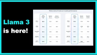
Llama 3 is here! | First impressions and thoughts
Elvis Saravia
Llama 3 is Here! #ai #llms #llama3
Elvis Saravia
Microsoft introduces Phi-3 | The most capable small language model?
Elvis Saravia
Microsoft introduces Phi-3! #ai #llms #microsoft
Elvis Saravia
Make Your LLM Fully Utilize the Context #ai #llms #machinelearning
Elvis Saravia
When to Retrieve? #ai #llms #machinelearning
Elvis Saravia
Training an LLM to effectively use information retrieval
Elvis Saravia
State-of-the-art open-source LLM judges #ai #machinelearning #gpt4
Elvis Saravia
Better and Faster LLMs via Multi-token Prediction
Elvis Saravia
AlphaMath Almost Zero #ai #science #machinelearning
Elvis Saravia
SWE-Agent | An LLM-based Software Engineering Agent
Elvis Saravia
[LLM NEWS] AlphaFold 3, xLSTM, OpenAI's Model Spec, DeepSeek-V2, OpenDevin CodeAct 1.0
Elvis Saravia
LLM-powered tool for web scraping #ai #chatgpt #engineering
Elvis Saravia
Learn about LLMs in this NEW course #ai #chatgpt #engineering
Elvis Saravia
[LLM NEWS] KANs, Gemma 10M Context, OpenAI Updates?, Automatic Prompt Engineering, Tokenizer Arena
Elvis Saravia
[LLM News] GPT4-o, Project Astra, Veo, Copilot+ PCs, Gemini 1.5 Flash, Chameleon
Elvis Saravia
Enhancing Answer Selection in LLMs #ai #machinelearning #engineering
Elvis Saravia
On exploring LLMs #ai #promptengineering #chatgpt
Elvis Saravia
Transformers Can Do Arithmetic with the Right Embeddings #ai #machinelearning #engineering
Elvis Saravia
[LLM News] xAI Series B, Codestral, LLM Guide, AutoGen Course, Symbolic Chain-of-Thought
Elvis Saravia
PR-Agent #ai #gpt4 #software
Elvis Saravia
Extracting features from Claude 3 Sonnet
Elvis Saravia
Has prompt engineering been solved?
Elvis Saravia
More on: CV Basics
View skill →


Related Reads
📰
📰
📰
📰
Want to get started with deep learning
Reddit r/deeplearning
Building a Deepfake Detector From Scratch — What Nobody Tells You
Medium · Deep Learning
Unfolding the Meandering Path: High-Dimensional Invariance and the Flat 2D Plane of Neural…
Medium · Deep Learning
Implementing Neural Style Transfer from Scratch: The Project That Started It All
Medium · Deep Learning
🎓
Tutor Explanation