SQL for Data Analytics – Intermediate Course + Project

Key Takeaways

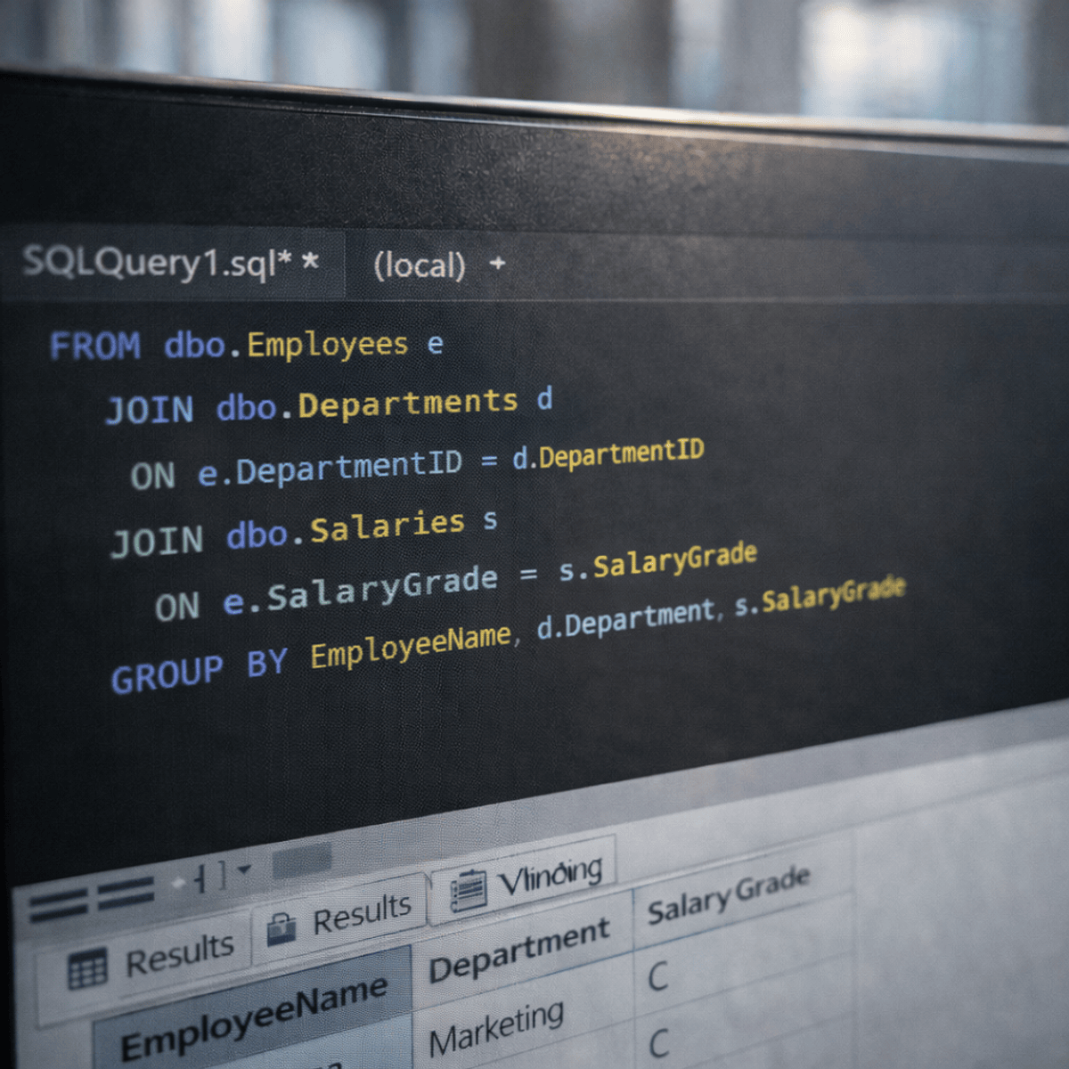
Data nerds, welcome to this full course tutorial on intermediate SQL for data analytics. This is the course for those that understand the basics of SQL but want to take it to the next level. Perfect for those that took my first course on this. Now, to master this tool, we'll break down more advanced SQL concepts in short 10-minute lessons. During this, you're going to be working right alongside me, completing realworld exercises. Following each lesson, you'll have the option to do interview level practice problems to not only prep you for the job, but also reinforce your learnings. And by the end of the course, we'll have used SQL to build a fully customizable portfolio project that you can share to demonstrate your experience. Now, SQL is by far the most popular tool of data analysts. For those in the United States, it's the top skill that's in almost half of all job postings for data analysts. And this only increases in demand for senior data analyst roles, coming in at two out of every three job postings. Now, in related data jobs like data engineers, it's almost the same, appearing in two of three job postings. And for data scientists, it's in almost half. Now, SQL or SQL is the language used to communicate between you and a database. It's my mostused tool as data analyst. Starting with my first job working for a global Fortune 500 company and even to my most recent role working with Mr. Beast. Yeah, even Jimmy uses it. This tool is so imperative. I use it all the time with Python, Excel, PowerBI, and Tableau to connect to my databases. So, over the years, I've been cataloging everything I found helpful with using this tool, and I put it all into this course. Now, you're probably wondering, who is this course for? Well, if you're unfortunate to take my first course, here's some items you should definitely know. Keywords used for data retrieval, functions and keywords used for aggregations and grouping, the different types of joins, and also unions, keywords used for logic and conditions along with date manipulation, data schema control, and finally subqueries and CTE. Now, as far as the math required to take the course, if you have a secondary education such as high school in the United States, you have the requisite knowledge to take this. We're going to be doing at most just some basic algebra and statistics. Now, let's get into the course structure. We're going to be breaking this down into two halves. In the first half, we'll have an intro that will get you set up and comfortable with the database we'll be using throughout the entire course. Next, we'll jump right in pivoting data using case statements. We'll be transforming and analyzing data using aggregation and also statistical methods. Then, we're going to get into intermediate date and time functions because frankly, you can't get away from date and time data in databases. We'll then wrap up the first half covering window functions. The most requested topic I've gotten by far on this covering basic and also complex aggregations. Now for the second half of the course, we're going to shift gears. We're going to not only install Postgress on your machine, but also we're now going to be working in these lessons to building our portfolio project. We'll start by setting up the database locally and installing a top editor for running SQL queries. With this environment set up, we'll build our first view. And this will actually help us solve our first portfolio problem. After this, we'll transition into learning the most popular functions to transform messy data to solve our second portfolio project problem. And then we'll wrap all this up with query optimization, understanding how to use keywords like explain to optimize queries. So, by the end of this, you'll have a real world project to showcase your newfound skills and demonstrate your experience. Now, I'm a firm believer in open sourcing education and making it accessible to everyone. So, this course is completely free. I've linked all the resources you need below, including the SQL environment and all the different files you need to run the queries remotely and locally. Oh, and also include my final project that you can also model after. Now, unfortunately, YouTube isn't paying the bills like it used to. So, I have an option for those that want to contribute and thus help support fund more future tutorials like this. For those that use the link below to contribute, you're going to get some more additional resources. Specifically, after each lesson, you're going to have access to interview level SQL problems. It will not only reinforce your learnings, but also prep you for job interviews. In here, you're going to get community access to be able to ask any questions to fellow students along with access to the queries and notes behind each lesson so you can follow right along as I go through it. Finally, at the end, you'll receive a certificate of completion that you can share to LinkedIn. Now, for those that have bought those supporter resources, you're going to continue watching the course here on YouTube, but then you can go to my site to actually work through all these problems, access to the notes, and access to community. All right, we're about to get into the first lesson. Before we do that, I want to cover some common questions and answers. Specifically, we're going to start with this one first. What database are we even using? Well, every year, Stack Overflow interviews a bunch of nerds to find out what are their top technologies that they're using. And 50,000 chose that Postgress was their top option to use and to use over the coming year. And according to this visual, it's not only the most admired, it's the most desired to learn database. So for this course, we're going to be using and learning with Postgress. Now that we know the database, how the heck are we going to be running these SQL commands? Well, as I mentioned previously, this course is broken into two halves, and we're going to be using an option for the first half that gets you up and running quick. Specifically, we're going to be using Google Collab, which is a free option, and it allows us to have an environment that we can not only load the database in, but also query it. I've linked this notebook below and includes all the code necessary to install this database and get into querying it. Now, don't worry if you haven't used Collab before. I'm going to break it down all in the next lesson, which for those that bought the course perks, you're going to get access to these lessons which are in a Jupyter notebook. For the second half of the course, we're going to shift gears and we're going to install Postgress locally on your computer and run all the queries from there. We're going to get you set up with PG Admin, which is Postgress's custom guey in order to interact with databases. But from there, we're going to get you set up with the most popular database editor, DBaver, which is used by over 8 million users. And this is where we're going to be running our queries. And I like this editor because it's not only free, but it also connects to a host of different databases. So, whatever you use and learn in this course with this editor, you can apply to other databases. Now that we know the database and the editor, what data set are we going to be using for this? Well, I present to you Cantazo, and this is a data set created by Microsoft used to imitate real business data. Jumping back into DBaver, we can see the erd or entity relationship diagram, and this shows how the data set revolves around sales data. That's the fact table. And then we also have four dimensional tables that relate to it. This is going to be great for analyzing business transactions in a real world scenario. We're going to go over everything you need to know for this after our Google Collab lesson. Now that we got that out of the way, let's get into some resources you have available, starting with those that have decided to support the course. First, I'm going to walk you through how to get access to the course notes, which detail all the different topics and code that I use within each lesson. And next, you're going to have access inside of the course platform to interview level SQL practice problems. After each lesson, I'm going to provide you with a bunch of different practice problems that range in difficulty for you to go through and test your skills. If you get stuck, feel free to jump in the comment section below and talk with other students in the course. Speaking of help, how the heck do you get help in this course? Well, you could jump into the YouTube comment section and hope somebody comes and actually answers your question, or you can get a really quick answer going to a reputable chatbot like ChatGBT. I use this bad boy all the time with my coding issues and it gets you an answer quick. All right, next question. Well, isn't really a question. It's more of a statement. People tell me all the time, Luke, this video is too long. I can't navigate it. Well, unfortunately, I think you don't know how. First of all, I include chapter markers for all the different lessons throughout this. The next is keyboard shortcuts. I like to use J and K in order to jump forward or backwards 10 seconds. And then finally, if you need more precise navigation, you can just click and drag up on the navigation bar of the video itself. And then you can do precise seeking. Pretty cool. All right, last question. Who helped build this course? And I'd be remiss if I didn't give a shout out to Kelly Adams. She was the brains behind putting together the lesson and also a lot of the practice problems for this. This course wouldn't have been possible without the help of her. All right, let's get into the first lesson. All right. In this lesson, we're going to be going over how we're going to be running SQL queries in this first half of the course using Google Collab, which is a type of Jupyter notebook. So, link below is a blank notebook and opening up. It's not fully blank, but it's blank enough to actually get started with writing SQL queries. Let's do a quick demo of how we're going to use this for SQL queries. First, I need to run this cell up top, and it's going to give me this warning that, hey, this notebook was not authored by Google. It's fine. It's run anyway. It's from me. You can trust me. It should take about 40 to 50 seconds to run this cell, which we'll go through more later in this video. Basically, it's loading the database and getting it set up for us to actually use. And now run SQL commands. So, inside this code cell, let's provide a command. So, we're going to begin by writing our command underneath this percent SQL syntax right here at the top. And I'll provide this query. Looking into the sales table, looking at those top 10 options. I can run it by pressing this play button or pressing shift enter. In less than a second, I have all the different results pictured below. If I want to run another cell, I can just come underneath it, click code, make sure that I add that percent sequel to the top of the cell. It's not going to work otherwise. And then run my next command that I want to right underneath this. All right, with that out of the way, we're going to now dive deeper into understanding what is Google Collab, what are Jupyter Notebooks, how to actually use these to run SQL queries, and what the heck is going on with all that code that I had in those cells. Now, if you have familiarity with using Google Collab already or already confident in using Jupyter Notebooks and you feel like any of this that I'm going to cover is not relevant to you, it's fine. Go ahead, skip to the next lesson. This is more focused on those that don't have any background with using Jupyter Notebooks. So, let's start with Jupyter Notebooks. Here I have a Jupyter notebook of this actual lesson inside of VS Code. Don't worry, you don't need to actually open inside VS Code. Just showing this for demonstration purposes. Now, personally, I love Jupyter Notebooks for performing analysis because not only can I have these text cells like are pictured right here, and then scrolling down even further, I can see that at the bottom, I have a SQL cell along with the SQL output. So, I love these because I can use SQL to extract out and analyze the data I need and then if needed use something like Python to visualize it. Now, moving into Google Collab, which you can see right here, I'm inside my web browser and this is that same exact file that I had inside of VS Code, but now it's here inside of Google Collab. And similarly, it has that same functionality where I can write Python code in cells along with using that SQL and the outputs of that below it. I really like Google Collab because it makes it super easy to share and collaborate with others. This isn't just a static document. I can come in here and actually run all the different cells inside of this notebook. And if somebody wanted to, they could come in and modify this query further. So right now, this one's only looking at years. Let's say we wanted to look at the actual total revenue. I could just add this line in the command, run it, and get the results right below. So super easy to collaborate with others. And now you may be wondering why are we actually using collab for running these SQL commands. Well, basically this code right here that I have in this cell that we're going to cover, I promise allows us to load in our database and for you to have access to the database immediately without having to actually install it locally on your own computer. So basically, we can get up and running with running all these different SQL commands really quickly. Let's start with a blank notebook to walk through this process of understanding how to use notebooks. If you navigate to collab.resarch.google.com, this is where we're going to start a new notebook. And it will have prompted you to log into Google at this point. Anyway, go and click this. So, it starts this new one which gives the title untitled zero. You can go up up here and actually change it. And I'll change it something like collab 101. Quick overview before diving into the center portion. Right here we have a typical menu up at the top to do a bunch of different options. And then we also have this sidebar over to the left hand side that gives us a lot of different options as well. In the center here is where the actual notebook is itself. And I can do things like either add a code cell or a text cell. If I wanted to, I could type into it. This is a text cell. I can also change the formatting of it by highlighting it and toggling it to being a heading. They also have multiple other options available as well. Whenever I'm done with this, all I have to do is press shift enter. And whenever I press shift enter, it then starts another cell, a coding cell below that. Now, in Collab, these are exclusively Python cells. We have to do some magic, if you will, in order to get it to run SQL. But you may not realize it, but you actually know some Python, even if you don't know it. I could do something like 2 + 2. Press shift enter. And what's going to happen here is it's going to run the cell of 2 plus 2. and then we get the results of four. Now, if I don't need certain cells, like this one up at the top, I just click into it and click the trash can. Similarly, I can do it to this one down below. Now, let's go over these menus. And for this, I'm going to be demoing it using the actual lesson plan notebook from this cuz it makes it more interactive to show actually the capabilities of it. Anyway, over on the lefth hand side, if I click this over on the left, I have the table of contents. Based on how I formatted all the different lesson notes, I can actually scroll through and see all the relevant topics. If I wanted to find something, I can just go in here, type fine of markdown, and as expected, take me to all the different markdown things inside of here. We also have other things like variables, secrets, and also files. That's more in depth. If you're using Python for this, you won't really need to use that. Along with these three at the bottom, also not going to be using as much in this SQL course. Now, up at the top in the file menu right here, file, edit, view, insert, everything like that's normal. Runtime is the one location that I find I'm actually using the most and find the most important. Anytime I'm opening a notebook, I'm going to be doing this run all. And I can also see that I can do this with the shortcut of command F9. And this will go through and actually run all the cells. down here at the bottom, it gives you a status update of what's going on along with the time it's taking so far. Now, scrolling through all these different cells, I can see they all executed properly. But sometimes we run into bugs and they're not running properly. In that case, we can come up here into runtime. And I recommend running this of just restart session and run all. It will prompt you if you need if you really want to do this. And yes, go ahead and do it. Basically, clear everything out and run it again. That's only if you're having problems. You shouldn't, but if you did, now you know. In this last section of the lesson, let's understand what is going on with how we're running SQL queries inside of this notebook. For this, I want you to actually open up that blank SQL notebook and load it into your window and you can follow along with me. If you haven't done it already, go ahead and up at runtime, click run all. So I mentioned earlier all of this code here which is in Python goes through and actually installs and sets up your database. We're going to walk through it really quickly. But the important thing to understand here is not necessarily the code or that you need to code it yourself. It's mainly understand what's going on behind the scenes. First it goes in and imports some important libraries that we need for this. Next, if it's in Collab, which we're in, we go in and install Postgress. So Postgress is actually running inside of this environment that we're inside of. It goes through and sets up a user, a password, and then from there actually installs the database itself, which you can get at this link right here. From there, we import in a SQL library in order to be able to run SQL commands. Specifically, it's called GPS SQL. And then with this JubSQL, we go ahead and load the extension. actually connect to this database that we loaded in from up above and do some other fancy things that help us get formatting and everything else set up properly. So, similar before below this magic command of percent SQL, I can write a SQL query. As I'm writing these SQL commands, you should have autocomplete come up. So, in this case, I have select. If I want to use it, all I have to do is press tab. And then once I have everything I need there, once again, I can press shift enter. Now, that magic command is really important. If I were to copy this, paste it below. One, I get all of this highlighting saying that it's misspelled and that they have syntax errors. And then two, when I actually try to run it, I get actual syntax errors. So, very important that you put these magic commands up at the top. Now, so people don't think I'm crazy, magic commands are the actual official language of this. And we're not only limited to SQL magic commands. They also have a host of other ones. Let's say I want to use this one of time it where it measures the execution time of the next line of code. I could type the magic command of percent time it. Some help pops up of what actually is going on with this module that we're actually using here, which is pretty actually useful. And then underneath it, I can put some Python in here. I'll just do something simple like 2 plus 2. Running this. Pressing shift enter. We can see that this special command provides the time of this took 9.93 nanconds. Now with these magic commands, you can also use just one percent sign and that means it applies only to the line that it's currently on. So in this case I could do 2 + 2 on this line. Press shift enter. It's still going to run it which in this case looks like it's a little bit faster. But if I actually had only one percent sign and let's say this is on another line, pressing shift enter, it's just going to output the four and it's not going to actually time it. It's not until I actually use two of the percent times and run it that it will actually time it. And now we're back up to 9.85 nconds. So I'm just reinforcing this because it's very important that you remember to do that percent SQL before any SQL command. Now, if you're nerd like me and you want to dive deeper into the documentation of JubSQL because of the brains behind that SQL magic man, you can a link below. All right, for those that purchased the supported resources, you now have some practice problems to go through and get more familiar with how to use Jupyter notebooks and SQL queries together. In the next lesson, we're going to be diving deeper into the database to understand all the different tables and what comes along with it. With that, I'll see you in the next one. In this lesson, we're going to be getting an intro into the database that we're going to be using for the entirety of this course, specifically the Contazo database. For this, we're not only going to explore why we're using this data set, but also the components about it, exploring all the different tables using things like the erd or entity relationship diagram. Now, we're going to use this lesson as a warm-up to get ready to get into using intermediate SQL. So during the course of this, I will be covering different past topics that you should know in order to get you up to speed as fast as possible if you haven't used SQL in a while. By the end of this, we're going to be covering a query from scratch in order to dive in to the most popular tables while using Google's Collab and some additional AI features to speed up your workflow. Now, the Contazo database that we're going to be using for this is based off of a data set from Microsoft which they've been using for years whenever they launch any products, specifically SQL products, in order for you to explore how to use the functionality of it. Anyway, this database is really robust because it contains a lot of different information in it such as sales transactions, product information, store details, and even date and time data. And this database is great because it allows us not only to explore all these different intermediate SQL topics that we're going to be using for this, but also it's based on a real world business set of data. So what you're going to learn in this course, you can apply to the real world. And so you may be like, Luke, how the heck do I get this database installed? Well, if you remember from the last video, we have this Python code up at the top that actually goes through and installs the database. The database or the SQL file for loading it. It's located at this link. And we go through this script right here in order to load it in to this collab notebook, which I've conveniently linked a blank notebook below that you'll be able to follow along any of the lessons with. So, this diagram shows via these lines between all these different tables how they are actually related. And there's actually a lot of columns inside of these tables themselves. So, we put these ellipses at the bottom to basically signify or symbolize all the different columns that are in it. So, let's get into breaking this bad boy down. We have a total of six tables in this contazo database. Specifically, our main fact table is the sales table, and this contains all of our quantitative business metrics that we're actually going to be analyzing and inspecting as we go throughout the course. So, it's probably the most important table you need to know. Then we have four related tables or commonly known as dimensional tables. These things have descriptive attributes that we can use in our analysis. So for things like store, we relate it using the store key and the sales and then stores table and the store database has information on well the stores. Similarly been said about the product and also the customer table. The date table is slightly different in that it relates to the different dates, specifically our order and delivery date. The last table in this is that currency exchange table, and it's not related at all to our fact table, and we'll show why in a little bit. Now, you may be wondering, how can you actually go through and see what this database looks like and understand what are the tables in it? Well, we're going to be exploring tools later in the course. Specifically, this is PG admin right here where I can visualize that erd and it shows how our fact table of that sales table is related to all those other different dimensional tables. Additionally, it's pretty nice because I have this Kazo 100K and I can go into something like schemas and then down to tables and further I can further explore all these other different tables as well, even looking at things like the columns for the sales table. But we're getting ahead of oursel. We'll learn how to do that in a bit. I'll teach you some shortcuts on how you can actually do something similar to this in Collab. So, let's get into running some queries. First thing we need to do is go through and actually run all the different cells in your notebook. Basically, get that database loaded into our environment. And so, we're looking to explore what are the tables in this database that we just loaded into here. I'm going to use Gemini for this. If it's your first time using this AI model from Google, it's going to prompt you with this privacy notice. Make sure you click continue. And I can prompt it this of what SQL query shows the tables in a database. What we can do is access all these different table names by looking in information schema which is a meta database and specifically using the data attribute the looking at the tables within it which is a table. Now for this you can either click copy cell or you can do add code cell. Now remember, we're going to have all the syntax highlighting issues because we're not or we don't have in that magic command we need to put at the top, specifically that percent SQL. So I'll just copy that from here, paste it up here, and then run this bad boy. So from this, we confirm we do have six tables in our database. And if I wanted to, I can convert this data frame to an interactive table like this. And then we also have this option to visualize it, which we'll be doing down later down the road. So let's explore first that sales table as that's the most important part of this whole puzzle. I want to see all the different columns of this. So I'm going to use select and then star. We're going to do this from that sales table. Now if you're noticing right now I have some autocomp completion happening right now. You see I typed sales and I have this underscore fact underneath it. This is the AI autocomp completion. Especially whenever I'm learning how to use SQL. I don't find this very helpful and actually quite distracting. So we can turn this off real quick. If we go into open settings and select under AI assistance, we can uncheck this option here for show AI powered inline completions. Whenever we close this, we can see no longer pops up. Now this is good enough query as is, but anytime I do a select star type thing, it's very resource inensive, especially if there's a lot of columns and rows. So with this, I'm going to limit this to just the first 10 rows. Then from there, press control enter. also don't need this query off to the side. So I'm going to close that. So with this sales table, we can see that it has all those different relations to those other tables such as the dates, customer key, sore key, and product key. From there, we have information on what is actually sold in this sale, specifically the quantity, the price, the cost, and then also the currency used, and its exchange rate. In our example at the end of this, we'll go through calculating what is the net revenue and how we need to actually multiply or use all this together to calculate that. Let's get through exploring these tables. Specifically, we're going to go with the easiest one first next of exchange rate. If you recall, our currency exchange table is in no rel way related to that sales fact table. But what the heck is in it? Well, exploring it, we can actually see that in it, it has a date column from currency to currency and exchange rate. Basically, it at a specific time in history, it tells you how you could convert a currency from one to another, what the rate you need to use that. Now, conveniently, our sales table automatically just includes this exchange rate, which was calculated from this table. So technically this table is only needed if you need to go back and dive into understanding the exchange rate and how it's trending over time. All right, we have four tables left and they're all the dimensional tables that related to our sales table. Let's start with store first. This one is related to that sales table on a store key and then has information on where this is located such as country, name of the store, even the size. Next up is our product information and it's related to that sales table on that product key. It has information on the product, specifically what is the name, who's the manufacturer, how much it even weighs, and what categories and subcategories it falls into. Next up is our customer table. It's related to that sales table on our customer key. And this has a bunch of information related to the customer itself, like where they're located, what their name is, what their birthday is, blah blah blah. Anyway, what you notice right here in the middle is we have these ellipses and that's because there were so many columns in this, it didn't show it here. Now, previously whenever we were looking for the tables in the database, we could run this on that metadata inside the information schema. So, what I'm going to do is actually I'm going to take this right here, command C this, and I'm going to paste it right into here. But for this, we don't want to use tables. We want to use columns. Running shift enter on this. This only gives us table name information. So I'm actually going to change this to select star. Run shift enter. So we can see everything available in this query. And inside of here I can see of this columns table. We have a table name and column name. So what I can do is I can now filter this for the table of customers. So I'll specify where table name is equal to customers. Running this again. Pressing control enter. Got a typo. It's customer running control enter again. So now I have a way to view all the different column names and it's not cut off and so we can see everything inside of it. But not really finding anything that great right here for now, but other stuff we'll use in the future. Last table to explore is that date table. This is related using that date column here to the sales table, order date and delivery date. Now, this table has a lot of different ways that you could aggregate all the different date data in here by looking at maybe day of week or month or year. So, this is great and all, especially if you're using a tool like PowerBI and you want to just grab something quickly in order to filter maybe for January 2015 data. But in this course, we're going to be diving deeper into using different date functions. And so we're not really going to rely on this table at all to get the data out because you won't always have a date table available in order to investigate things. So basically just ignore this bad boy. Now let's wrap this lesson up by getting into an investigation of how we can use all these tables together for a common example. So let's say my boss who's not so good at SQL comes to me and wants to get some different revenue data that has information about customers and also products they're ping purchasing and whether they're of different high value or low value items. So we're going to walk through this example calculating the net revenue for this and how we can put this all together using all the different tables. First thing we need to do is calculate net revenue. So let's look back at that sales table. We're going to use that same query as below and we get this table that we saw previously. Now, for this, how do we want to actually calculate that net revenue? Well, in order to do this, we need to use the net price. Now, you'll notice from this, the net price is less than the unit price. That's because the net price is the price after all the different discounts, promotions, or any adjustments. So, basically, it's what we actually charge to the customer when they pay for the product. And with this net price, we need to multiply it times that quantity. So what I'm going to do is put a comma here. Go to a next line and say we want to multiply the quantity times the net price. And we'll say this, we'll label this as the net revenue. Now when I name variables or when I name new column names, I'm going to put this underscore between it. I just find it easier to read the naming convention that Kazo's database is using. And looks like I have a typo, which is pretty good that we hit this right now because this is how I'm actually going to go through and troubleshoot this. First, it will tell me that there's this runtime error anytime I'm running a query. You can just ignore that. You're going to be seeing that all the time. But it actually points this carrot here to where the issue is. Specifically, it's point to this line and it has to deal with quantity is not spelled correctly at all. Running this again, pressing controll enter. Okay, we actually have it now. And over to the side we have that net revenue. Double checking this. It looks like all the numbers are actually getting calculated correctly. There's one last step to do and that is we need to convert it to a common currency. Right now you can see that they're using pounds here and then US dollars below. Basically we're going to use it all the same. I'm in America so we're going to be using US dollars. All we have to do for this is just multiply by the exchange rate. Gone ahead and added it in. And now we can see that it is in fact adjusted for what it needs to be. Now we're going to be adding customer and also product information using this customer key and product key. But this table's already getting sort of large. So I want to condense it down to different columns I'm for sure I'm going to use. And really the only other thing I care about is order date. So we'll go ahead and simplify this table down to this. Next we'll move into our second of five steps. And we want to filter for our recent sales. Specifically we want things from 2020 and greater. For this, I'm going to use a wear clause. And I want this for that order date that we have in that sales table to be greater than or equal to January 1st, 2020. Now, let's go ahead and try to run this. And it looks like it works. Now I would say in order to be safe if you're ever working with date data that you're not sure if it was converted to the date type specifically in Postgress you can use this colon operator and then specify the data type you want to use for this in this case date. So order date is getting converted or cast as a date. This is going to work just the fine but just a tip for you. All right, next thing my boss wants added in is the customer info about who ordered that order. Now, in order to do this, we need to use a join. And there's four major types of joins. Left join, right join, inner join, and then full outer join. In our case, we want to perform a left join because table A is our sales table. And we want any related data to that A table in the sales table returned from that B table or customer table. So, let's add this left join. We're just going to go between from and where. I'll add in a left join. We want to do this on the customer table. We're going to give it the alias just C to make it easy. Similarly, I want to give sales an alias as well. I'm actually going to bring this down and then indent this over. I'll give this the alias of S. Now, for this left join, we want to do this on from the sales table, we want to use that customer key. And then from the customer table, we want to use customer key. So we're going to use good actual naming conventions here. I'm going to add that s dot to the front of order date along with the front to quantity, net price, and exchange rate. Now I'm going to go ahead and run this to see if it actually works. And it looks like it works. We don't have anything from the customer table. I'm going to go ahead and add in all the different columns by doing basically a C.AR notation to bring all those in. All right. So from this list I can see there's a few different columns we want that my boss has told me about specifically we want to get the given name or first name surname country full and then also the continent that they're from. All right second to last step we need to add that product information in and similarly we're going to be forming a left join with this. We'll give that product table an alias of P and we'll be connecting it on the product key of the sales table and the product table. Once again, I want to see everything from that product table. So I'll do P.star. Running this control enter. I can see that we connected it properly with all the different product information. Once again, I don't want all the different columns associated with this. only want to select few does my boss specifically these four columns of product key product name category name and subcategory name all right so looking pretty good with this only one last step to do and we'll have all the information we need specifically we want to look at whether a customer is high value or low value looking at the net revenue we want to basically bin these customers into whether they're spending less than $1,000 or greater greater than $1,000. In order to accomplish this, we need to use a case when statement and we're going to add it in at that last column right here. So, we'll say case when we want to look at the net revenue, but we can't use an alias inside of the select statement because it's not necessarily defined yet. So, we just need to take all of this below, paste it in here, and say greater than 1,000. And in that case, we want to say that it is high. else we want to say that it's low. So we can end this and then we're going to use the alias for this of high low real original. I know let's run this pressing control enter. Inspecting it we can see that our formula is working for those values that are greater than a th00and we're marking it as high. So this has everything that we need in it for my boss. Remember right now we're doing this limit 10. We actually need all the different data in it. So I'll go ahead and press play. Looks like we have 124,000 different rows in this. And if I want to export this to my boss, I could click this here in order to convert this into this type of table. But what's really convenient about this is I can now copy this entire table, which allows us to either export to a CSV, JSON, or even markdown. CSV is most common, so I'll use that. All right. So now that's our initial dive into this Kazo data set. We now have some practice problems for you to go through and get even more familiar with this data set, working through some problems. In the next lesson or the next chapter, we're going to be diving into using the case statement in order to pivot data. Super exciting. All right, with that, see you in the next chapter. Welcome to this chapter on pivoting with case statements and specifically we're going to be using statements like case when and aggregation in order to pivot data. But what the heck is pivoting data. Let's take a look at this simple example focusing on that first table first. Typically our data comes in a long format and in this case we have an example of a columns of date, category and sales where we have different categories of A and B. It's very common to pivot things such as on the category here of A and B. So that way we get to more of a wider format as shown below. This is not only easier to read and understand and analyze but also easier to visualize which we'll be doing in this. So, what will we be covering in the lessons in this chapter? In this lesson, we're going to be focusing on understanding the basics of using aggregation methods such as count and sum in order to pivot data. We'll use count to analyze the number of customers per region. And then we'll use sum to calculate the net revenue based on different categories in different years. In lesson two, we're going to build this up further and start looking at statistical functions such as min, max, median, and average. For this, we'll get into an example of calculating what is the median sales across categories. Then finally, in lesson three, we're going to jump into advanced use cases of case statements. Specifically, we're going to be looking at things like segmentation. We'll learn how to analyze by multiple and conditions in order to look at things like bucketing for certain years based on revenue. And then similarly we'll use multiple when conditions in order to analyze different bucketing of revenue tiers and see how they apply across different categories. Now I just showed a bunch of visuals and the goal of this course is not learning how to build or make visuals which I will show in this but really I want to be able to show that hey with these insights that we're gaining you can take it a step further and visualize it. All right with that let's get into it. In this first example, we're going to do a review understanding count, but also distinct count in order to calculate the total number of customers per day in 2023. This will be the final table that we end up getting. As always, if you want to follow along, open up that blank SQL notebook and run all the cells in it so we can get started. So remember, we want the total number of customers per order date. We can uniquely identify this based on the customer key. So add a select statement. From there, I'll add order date followed by customer key and then we'll get this from that sales table. Let's start with this first. So, as we can see from this, we have this is the first of 2015. We have duplicate customer keys, but then we also have a bunch of different ones. We're going to start simple first. We're just going to do a count of all the customer keys. So, I'll wrap customer key and count and provide it the alias as total customers. Let's run this. And this isn't going to work, right? because well we need a group by right so adding that group by statement we'll add in we want to do this by that order date and then run this again all right so now we have the order date by total customers right now I'm noticing that the dates are not in order so I'll add in an order by order date and not too bad but remember previously whenever we were actually looking at it we could see that customer key is actually duplicated we want to find the unique customer so we want to use something like distinct So going back up into our original query, all I'm going to do is add in distinct in here and then run control enter. And now those numbers are going to drop, right? Because they have a we're going to remove all those duplicates. Last thing we need to do for this one is just add a wear condition for filtering for dates in 2023. So I'll add an order date. And for this, I recommend using the keyword between. So we don't have to do that greater than, less than, all that kind of mess. and then putting in between January 1st, 2023 to December 31st, 2023. Running this, we can actually check the contents. Yep, January 1st to December 31st. One quick note now on visualizing this, you can use this button right here and actually select it to go through and draft different visualizations to try to understand what is going on here with the data. What it will do is it will give you different previews. In our case, this is time series data. So I know that's the best choice to use for the visualization. Whenever I go to select it, it will autogenerate all the different Python code you need in order to visualize that data. And then all you have to do is click add cell. And then running this, you can actually visualize it in more detail right below. So that's why I really like Collab for this is because it has Gemini implemented into it. makes it super simple for you to just go forward and actually visualize this. All right, let's now get into actually pivoting using count as an aggregation. And for this, we're going to be looking at something similar from that last example, understanding how many daily customers we have, but broken down by region, specifically three continents of Europe, North America, and Australia. For this, we're going to be getting this final table where we have things like order date in the leftmost column and then we have the customers based on the different regions in their own individual column. First things first though, what continents do we actually have available inside of our database? It's underneath the customer table. When we run this, we can see as a previous report in got Europe, North America, and Australia. So let's go forward with actually adding this table into the query that we just made at that last example. In order to do that, we're going to be performing very commonly a left join. And that'll be with the customer table with an alias of C. And we'll do this on our customer key. And what we'll need to do now cuz we have two tables in here, we'll need to assign an alias also to our sales table and then also to all those other different columns that come from the sales table. Running this to make sure that the error there's no errors. There are accidentally messed up order date. Run this again. Okay, everything's working fine now. But now we need to create individual columns for total customers based on continent. So how are we going to do this? Well, let's focus on this syntax right here. We're going to be using the count distinct that we use as we used previously. And inside of this, we're going to be throwing in a case when statement. It's case when a condition then what the output we want it to be the column in this case and then end and then finally assigned an alias. So I'm going to go ahead and copy this right here and I'm going to insert it in the next line underneath here. But we need to go through and actually fill it out. So the condition is we're looking for if it equals a certain continent. So for the continent from that customer table, we're going to see in this case if it equals to Europe and specifically the column that we want from this is then that customer key. So I'll go ahead and put that in. And this one will give the alias in this case called EU customers. Let's try this bad boy out. And bam. Now we have our European customers in here. Let's go ahead and add the other two as well of North America and Australia. All right, I got those in as well. Have the North America and then also the Australian customers. Go ahead and run this. And scrolling down, we can see that based on the total customers, the Europe, North America, and Australian, they do add up to this line right here. So that field of total customers is now somewhat redundant. I'm going to go ahead and actually remove that. And this will be our final query. Now visualizing this one similar to the last one. This one I find especially has multiple different columns in it. The visualizations it provide aren't that good. Specifically it is here in these time series but it's broken up to where this one's Europe, this one's North America, and then this one's Australia. They're not all on the same graph. So unfortunately Gemini in this case is not that strong in producing graphs. If you really want to visualize it and you want to know my method for it, all you have to do is go ahead and click that table. And then remember, you can actually copy it. And this is going to copy the table to your clipboard. So this contents right here, I want it as a CSV. I'll go ahead and copy it. And we'll need to put it into some sort of document because it's pretty long. So you want to put into a document such as CSV. So on Mac, I'll put in something like Textit. Um on Windows, you'll put into something like Notepad. I'll just paste the contents in using commandV. And then from there, just save it inside your favorite chatbot. In my case, I really like chat GBT. You could use Gemini Claude, whatever. I'll give it the simple prompt with the actual document of visualize this as a line chart. And then with it visualized, we can actually I like going in this interact mode on ChatGpt. We can actually go through and you can see both the all three of these regions along with visualize. If you want to download the graph, you can just click it there. Last example for this lesson. For this one, we're going to be looking at using the sum function with case when in order to look at what is the total revenue by category. And we're going to be using that case when in order to look at 2022 verse 2023. This is the final table that we'll be creating where we have category in the leftmost column and then we'll have the total net revenue for 2022 and then for 2023 right next to it. Now for this I don't want to start from scratch. So I'm going to do take this last query that we took right here and then paste into c