Image classification from scratch - Keras Code Examples

Key Takeaways

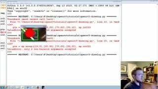
welcome to the henry ai labs walkthrough of keras code examples keras has provided 56 code examples implementing popular ideas in deep learning this ranges from the basics such as simple mnist and imdb text classification all the way to cutting-edge research ideas such as knowledge distillation supervised contrastive learning and transformers we'll also explore fun generative examples like variational autoencoders and cyclegan my contribution to these code examples is to explain every single line of code in each of them walking through each of the individual keras examples i'm not the author of these code examples please consider starting the github repositories to show support to the original authors as a quick preface to the video here's what you will learn from this video you'll learn how to download a data set from a link using shell commands in a collab notebook this data set will now be on the disk and we have to pipeline it from the disk into the working directory to pass it to a keras model you'll learn how to do this with the image dataset from directory keras function we'll see how to visualize data and then importantly we'll see how to define a pre-processing and normalization pipeline where you have two options to either pre-process the data on the cpu or define it as a part of the model where this happens on the gpu then you'll see how to build a model particularly the exception architecture using skip connections and how to visualize the model using plot model then we'll train the model explaining the epoch step through and then we'll show you how to do inference on a single image of a cat and have it classify it as a cat rather than a dog the first example is image classification from scratch this example is going to show you how to take a data set of images stored as jpeg files on the disk and load it into keras to train an image classification model in this case we're demonstrating this using the kaggle cats vs dogs binary classification data set this just means assigning a 1 for a cat and a 0 for a dog the tutorial also describes how we're not doing this with pre-trained weights or pre-made keras application model later on we'll describe more what this means this reference is using transfer learning where you take say resnet 18 resin at 50 mobilenet one of these pre-trained convolutional neural networks and then using that to initialize the parameters of your neural network for some downstream task and generally that works much better for particularly for small data sets but in this case it's showing you how to do image classification from scratch from scratch referencing a random initialization of this deep neural network so we're going to use the image data set from directory utility from keras in order to show you how to pipeline this keras image pre-processing where you take the images the jpeg files and then you pre-process them and prepare them to get them into the working directory of batching them and pairing training loss updates for deep neural networks we'll also look at some image standardization and data augmentation in this pre-processing pipeline so the first lines of codes are import tensorflow is tf from tensorflow and porkeros from tensorflow.keras import layers this is the last time in this code series that i'm going to explain these kinds of imports basically all you're doing is you import the tensorflow python library and then you alias it with tf what this means is that when we're going to be calling functions that are written in the tensorflow software package we're going to use tf dot and then access the attributes or the functions of the tensorflow library similarly keras is a library on top of tensorflow and we also do from tensorflow.keras import layers so this syntax from import layers compared to import as tf just means that we'll be doing layers.dense or something like that for example if we wanted to have the same kind of syntax we do import layers as l or something like that but this is the standard syntax of how people import tensorflow keras and the layer so this is the last time in the keras code series that will explain these basic imports more interestingly now let's download the data set so this syntax where you use the exclamation mark this lets you use the terminal commands in the google collab jupiter notebook so you do something like exclamation mark ls to list the contents of the current working directory in this case we're using the exclamation mark curl to download this file from the internet so we hit run on this code and it runs the shell command to download this data set so as described this is a 786 megabyte data set of these jpeg images of cats and dogs that we're going to be training our image classifier so this isn't a very big data set we see that collab is able to access the data set in about seven seconds this probably depends on my internet speed as well and this may vary for how long it takes for you but overall downloading 786 megabytes of data across the internet it usually isn't that much of a bottleneck so if you go into the jupyter notebook interface you now click on this folder icon and you can see the new file that we've just downloaded so this has now appeared in our directory because we just downloaded it with this curl shell command so now we do is we have this zip file and we're going to unzip it so that we can get the uncompressed jpeg files we see now we have this pet images folder that we have our cats and our dogs and if you like you can click here and you could download it download this onto your local machine if you want you could go into the cat folder and you can find the individual cat image and download it so we also have a quick browser interface in our collab directory if we want to view these images so for example we click on 10.jpg then we view this cat image on this side shell of our collab interface from google collab so now we'll exit out this folder folder thing and go back to our original notebook so we can also have the shell command ls pet images this is listing the directories of that ped images folder and we have two folders cat and dog so the next line of code is about filtering out corrupted images so the idea of this is that we're scraping this data set from this web link we have this https downloadmicrosoft.com download and some of these images are corrupted and they're not formed as jpeg images so we want to filter out the badly encoded images by looping through this and particularly looking through the as bytes embedding so this is a bit more advanced than our high level overview of keras and tensorflow is concerned but overall what this is doing is it's just a way of filtering out bad files from this web scrape so some of the lines of code you import the os library use this number skip so that we have a sense of how many of these images have been corrupted we do the syntax of four folder name in cat dog meaning just cat dog this is the for loop we use the folder path as os.path.join os.path.join basically just concatenates pet images with cats would be pet images forward slash cat and then pet images forward slash dog so now we do is for file name and os.list directory folder path we pass in the folder path pet images cat and then we loop through each file name in that folder we join the path so that we can open this file and then we check what kind of encoding it's been so if it's been encoded with this jfif encoding then we're going to increase our number of skipped and we're going to remove it from the file path so os.remove that's going to delete a file so you have this os this is your python interface to your operating system and you can use commands like os.remove or os.lister to traverse the directory and make actions on the files so now we're diving into the first functionality of the keras library this is the tensorflow.keras.preprocessing.imagedataset from directory image dataset from directory is one strategy of loading datasets that are stored in the local directory on the disk into our current workspace to load it into our deep neural network or just any kind of training whether we just want to plot the images or do any kind of normalization statistics anything we want to do with our data set we can use the image data set from directory function to access it from this disk so some of the things we do we pass in the image size this means the height by width we have 180 pixels by 180 pixels we're going to be passing in batches of 32 images to train our deep neural network we're going to access the data from directory this is the name of the folder pet images the validation split we're going to hold out a subset of our data so that we can validate our hyper parameters and evaluate our model performance and then we seed this so that we can reproduce the same results every time so there might be there's randomness with respect to how it's going to split the data you pass in a seed such that you know that you're working with the same sets of data every time you run experiments this is really important for once you get into research or you're just overall trying to see what works and what doesn't make sure that you seed it so that you the results of your algorithms that you're testing are actually due to the new algorithms not because you've had a random different split of the data and that's really conflating the results that you're seeing with your experiments so we also pass in the image size argument and the batch size argument and then we similarly do the same kind of syntax for our validation set our next block of code is about visualizing the data with the matplotlib.pi plot library so what we're doing in this line of code is we define our figure plt.figure we just define the size of the figures 10 by 10 and then for images labels in train ds dot take 1. so train ds is the name of this object that is storing the parameters of our tf.kerasa preprocessing.image dataset from directory so dot take is how you sample the next image so we do four images labels and train ds.take each time you ask it to dot take and then one it will return to you another image from the the pipeline of going from disk into the current python workspace so now we're looping through a set of nine images and we're going to define the plt.subplot so this is the syntax for taking matplotlib and not just plotting one image but plotting this three by three grid of the images then we have this plt.image show the images you convert it into numpy so we take this image and then first we have to convert it into a numpy array so it might be loading it from the disk just as a jpeg file or you know maybe it's a pil image i don't know exactly what it is before it gets passed into this numpy but we do dot numpy to chain into numpy you could also convert any kind of tensor into numpy like this and then this is how you input it to matplotlib so matplotlib takes in numpy arrays and plots them with this i am show syntax so overall we get this nice visualization a great way to start our models is to get a sense of what our data looks like particularly when working with computer vision and images now we'll get into one of my favorite topics in deep learning which is data augmentation image data of augmentation are these transformations we make to the images that preserve the semantic label so for example we can rotate this dog image 10 degrees as shown in this random rotation hyperparameter 0.1 or we can horizontally flip it and it's still a dog there's no way to rotate the dog or horizontally flip it such that it becomes a cat so this is the syntax for defining our data augmentation pipeline in keras so we do keras as sequential and we have layers.experimental.preprocessing dot and then we have the set of implemented data augmentations in the keras library so you can consult the keras you go to the keras documentation you go to pre-processing and you can see all the different data augmentations that you can use right off the shelf to augment these images and then get more juice out of smaller data sets and also to other things that data augmentation has been applied to like training gans with limited data or contrastive learning to name a couple other examples so in this case we define random flipping and random rotations and then we use this and we can pass it into this batch remember that train ds.take is the tensorflow keras syntax for sampling the next image from our data loader if you're familiar with pytorch you know that syntax of data loaders this is the same kind of idea trainbs.take1 so we do is we take each of these images and we're going to pass it through this sequence of data augmentations and now we can get a look at what this image looks like so we see these cats rotated and horizontally flipped in this case you see an example of this one and this one is an example of a horizontally flipped image the next step after applying data augmentation is to standardize the data so as it is these rgb pixels are in the zero to 255 range and this isn't good for neural networks what we want to do is standardize these values into the zero one interval by using the rescaling layer so the tutorial describes two different options to pre-process the data so there are two different ways of doing this in keras so option one is to make it a part of the model so what this means is we have our data augmentation layer we first have our inputs layer where we have keras that input shape people's input shape this is where the 180 by 180 rgb cat or dog image would be inputted then it would go through a data augmentation layer and then would go through a rescaling layer now the other option is to do this before you even define your model so the other way is to take your trained data set and apply this dot map syntax you define this lambda function which is a quick shorthand of saying take x and then y which is the label and then return the data augmentation transformation of x and then label this training equals true this is something to do with the way that it's batching up the asynchronous and non-blocking batching under the hood this training goes through don't worry about this particular part of this for now all that you need to understand for now is that there are two different approaches doing this you can either apply the preprocessing as a layer in your model or you can do this offline and then define your model so you're passing in data that's already been rescaled and augmented to your model compared to implementing it as a part of the model okay so hopefully this made it pretty clear there are two options of doing this and really the difference is going to be more at scale it's going to be uh they're papers that look at things like how you're exactly batching and then what happens on the cpu what gets moved to the gpu with respect to pre-processing data but for our sake of this cat versus dog thing this isn't going to make much of a difference but if you are doing this at large scale experiments you should be more mindful of how this is uh what's getting preprocessed on the cpu and then how this data gets moved from cpu to gpu and all that kind of stuff but that's going to be a little out of the scope of this current tutorial so the next step is this pre-fetched buffered prefetching so again this is more of the technical under the hood of exactly how data goes from the disk into our working memory space for the sake of training these models so i wouldn't but i wouldn't worry about this too much depending on what level you're at if you're dealing with really massive data sets though i would definitely pay more attention to this compared to if you're just starting out with image classification so now we'll get into the start of the show which is building the model building a deep neural network with the keras library so we're going to build a small version of the exception network so this is one of these you can read one of these research papers that tells you exactly what it is about the model architecture in the exception network but hopefully it'll be clear enough from this code that you won't need to actually consult the paper so quickly also in the beginning they motivate using keras tuner keras tuner is a strategy for optimizing the hyper parameters so to jump ahead a little bit we see how we have these hyper parameters for example when we have a two-dimensional convolutional layer this uh 32 feature planes could be an example of one hyper parameter same thing with 64 feature planes as well as this loop through different 128 256 these are all configurations of the hyper parameters of a neural network so the article begins by motivating keras tuner as a way once you're a little more advanced and you understand this code and you want to start finding the optimal configuration of these parameters for your deep neural network so as we mentioned previously with the two options of doing normalizing the data this is taking option one so in option one we have these two different layers and we make it all a part of the model so that we can just get the raw images and then the model object will process the entire data so we have the input layer kerasine input shape equals input shape which is the 180x180 then we have that data augmentation block which we defined up here this sequential processing of random flipping and then random rotation and then we have a keras dot layers that experimental.preprocessing the rescaling layer that's going to normalize every pixel value to lie on the interval between 0 and 1. so now we start to define our convolutional neural network so some of the key ideas here is making sure that your feature maps haven't run out out of bounds or out of space so to say so this isn't really going to matter too much with 180 by 180 images but say you're playing with the c410 data set where you have 32 by 32 if you use 3 by 3 convolutions with a stride length of 2 you're going to decrease the size the spatial resolution of the feature map so it might go from 32 by 32 to 28 by 28 and so on and if you just stack these layers together with no sense of what you're doing you might eventually have like a zero by zero thing and it'll obviously throw an error and the whole thing will break so be mindful of this stride equals two this is down sampling the spatial resolution of the feature maps and you don't wanna run out of the height by width of the feature maps so what we do here is we define uh padding this is a padding you add zeros to to keep it as the same dimension to preserve this spatial resolution uh you have this keras syntax of taking the previous layers output and then passing it in through x equals and then you have this chaining where you add the in parenthesis x and you do this on and on you stack these blocks together this is the way that we define these convolutional networks most neural networks are just done by repeating these blocks over and over again like even the transformer neural network is done by stacking these self-attention blocks on top of each other say eight to twelve times so the way this exception model architecture works is we begin by taking the input and passing it through two blocks of convolution batch norm and relu activation now we're going to use a residual skip connection so resnet's this residual connection what it does is it projects the feature maps at say layer l minus one up to layer l plus one so that the bottleneck of going from l minus one to l to l plus one is alleviated by having the skip connection ahead and it helps with preserving information flow in deep neural networks so if you're informat interested in that i recommend checking out the resnet paper one of the most influential papers in deep learning so another thing to note is the syntax of looping through and constructing the neural network through a for loop so we're seeing this remember the syntax of passing in the x of the previous output in order to chain these function calls together and construct this object of the deep neural network in python code so we do is we step through each of these feature map sizes and this size is used to define the number of feature maps so here another thing to note is we're using a separable convolution 2d the separable convolution describes this technique of making it more memory parameter efficient but i wouldn't worry about that too much for now and also just using keras you can just treat this as a black box separable convolution 2ds these are more efficient convolutions compared to just the standard layer but see how this code is looping through this array of different filter map sizes and then passing it in to construct the object by passing in this size hyper parameter so you loop through four times constructing these different layers with the residual connection then you take all that output put it through another convolution batch norm activation and then we do a global average pooling so average pooling is where you take a neighborhood of two by two or you know any kind of neighborhood and then you take say the max value or in this case the average value so it's one way of reducing the spatial resolution of features in a convolutional neural network and then we append our activation layer so an activation layer and now at the classes level this is where we've processed these cats or dogs and now we're finally making the decision is this a cat or is this a dog and this is done by having a feed forward dense layer that has this number of units so in this case it's going to have one unit and it's going to have an activation function either sigmoid or softmax so sigmoid is a function that will turn it into either zero or one whereas softmax will normalize the logits into a probability distribution so softmax and sigmoid it is worth noting that these are slightly different ways of transferring this output logic into a class label prediction so then all in all once we define this model we return keras.models the inputs layer and then the final outputs layer where we take in this final classification logits and pass it through the activation function so in this function we've defined this make model that takes in an input shape of an image and the number of output classes in this case two cat and dog and it produces this model architecture so now we use the keras.utils.plot model to view our model so as mentioned previously we begin our model with the input layer then two blocks of convolution batch norm and activation so what this looks like is we have the input then we have the convolution batch norm activation convolution batch form activation and now we get to this for loop where we're defining these skip connections so with the plot model we get to visualize what these skip connections look like we've taken this previous activation feature maps of 90 by 90 by 64. so this means we have 90 by 90 height by width of this feature plane then we have 64 such planes so this goes into this layer where we pass it through activation convolution 2d batch norm and then three of these layers and then we have this convolution and then this skips ahead to be added with this feature map so this is the idea of skip connections we have this branching in our architecture and then it skips ahead and this is a dramatic improvement in information flow has been one of the biggest breakthroughs in designing deep neural network architectures so now we've defined our data we've defined our pre-processing pipeline and we've defined our model now it's time to actually train the model so first we define the number of epochs this is the number of times we want the model to step through the training data so we have training steps and then we have epochs a step would define an individual batch of these 32 images whereas an epoch generally refers to the entire set of cats and dogs and each time we step through the entire set of cats and dogs compared to just an individual batch so in chaos we have these callbacks callbacks are an argument you pass to the model.fit function as something for it to do at the end of every epoch in this case we're using the keras.callbacks.model checkpoint so what model checkpoint is going to do is it's going to save our model weights this is really important for all these experiments we're going to want to have a copy of our model before maybe the training is going to collapse or maybe we want to repurpose this model for transfer learning or maybe we just want to do some kind of experiments where we want to have a copy of our model weights so that we can load and save our model pick it up from where it previously was and this is especially important once we you know these state-of-the-art deep neural networks they're trained for like two weeks so you're training these models for a seriously long time and an important thing to do that especially if you're relying on these collab interfaces and cloud run times is make sure you're saving your model weight so it's extremely important so now we're going to compile the model we pass in the atom optimizer with this hyper parameter on the learning rate we have our binary cross entropy loss accuracy metric and then we pass in model.fit with our trained data set number of epochs this callback function and our validation data so when you run model.fit you get to see the current step of the model training in this case 6 out of 586 this means it's currently on the seventh batch of 32 examples and we'll have to do 586 batches of 32 in order to step through the entire cat verse dog training data set that we have on disk another cool thing about keras is it gives us the eta bit and built into the modeled outfit the eta is the estimated time until it's finished with this entire epoch in our case an hour and 15 minutes which can be incredibly frustrating 50 epochs is going to take us you know 50 hours about and this is the current loss this is the current accuracy of the model on the training set so this is what it's doing on the training set and then once it finishes the epoch the keras callback will tell us how it's doing on the validation data so in this case we see that it's taking an hour and 15 minutes to step through the data and this is because we're currently running on a cpu so now let's re-run switch this into a gpu and then re-run all this code and see how much faster this is so now we're running this on one of the gpus provided by google collab this is much faster compared to the cpu look at how it's just speeding through the batches of data this is a dramatic difference from the runtime that was previously shown when using the cpu so google collab has some really high power gpus if you're willing to pay this is the 10 a month subscription gpu which is uh the difference is usually like a tesla v 100 compared to say a t4 if the t4 is still fast if you're not paying for it but the tesla v100 it does have more memory it is a bit faster so i personally think it's worth it to pay for google collab pro but either way you see this huge speed up compared to these graphics processing units compared to cpus this is a very important thing to note throughout all of training deep neural networks they run much faster on gpus because you can parallelize the computation on these giant neural networks which is this forward pass with these big matrix multiplications so we see as we start the second epoch we'll get a good look at how long it takes to get through each epoch so we see we finished the first one and now what it's doing is it's calling this validation data callback it's going to give us our validation performance we see in this case we have 62.7 accuracy on the validation set and we have our accuracy and we also had this model checkpoint so we can go to our folder and we see here save at one this is what model checkpoint does at the end of every epoch it's going to save the model weights so this is the current frozen weights of our model after it's done one epoch of training so i'm going to stop this training and we're going to go right into this following code where we're going to run inference on new data so now that we've trained our model we want to run inference on new data we've trained a deep neural network and now we want to deploy it into the wild to classify a given image and tell us whether it's a cat or a dog so the first thing to note is that certain layers of our deep neural network can be inactive at inference time compared to training time we use data augmentation and dropout regularization to prevent overfitting with respect to fitting our deep neural network on this data but during inference time these layers provide us no utility so we're doing in this code is we load this individual image of one cat we have passing the 180 by 180 image size we pre-processed this image to make it a numpy array we use tensorflow.expand dimensions this line of code is how you pass one image through the to the deep neural network because the deep neural network is used to taking in batches as input size so you have to use this special syntax in order to reformulate the tensor of an image into a tensor of a batch size dimension so it's like zero by three by 32 by 32 if it's a c410 image in our case 0 by 3 by 180 by 180 you have to expand the dimensionality so that it's compatible with the input to the deep neural network so now our model is going to run model.predict on this image array we see our score predictions this is how much weight the model had put on each of the classes it thinks this image is 80 cat and 19 dog so this is how you make predictions with a new image having a trained model so thanks for watching this first walkthrough of image classification from scratch from keras examples this repository shows you how to load a jpeg image data set from the disk into the keras workspace how to download this data set from a web link using the curl shell command unzipping the zip file and then seeing working with the directory to make sure you have the right data set how to get out corrupted images from some bad link or some kind of bad data set this is how you basically process these files in python if that's the situation you find yourself in so now this is the syntax for loading an image dataset from directory this is one way of getting data from disk into the workspace for fitting these models this is how we visualize our images using matplotlib this was our strategy for applying data augmentation and how you use it using built-in keras functions how you visualize some examples of what data augmentation is doing to the data standardizing the data so it's between zero and one two different strategies for basically the key idea is efficiency with respect to the size of your data sets whether you want to do pre-processing on the cpu or on the gpu so if you do make it a part of your model this will happen on the gpu compared to if you pre-process it and then pass it the model or you do this on the cpu but again this only really matters if you're doing this at larger scale experiments so we batch the model we make our model this is one way of doing the skip connections and one syntax for learning how to construct the deep convolutional neural network and then visualizing the model using kerasa utils.plot model then we looked at how to train the model how to define the epacs callback epochs callback functions compile the model model.fit and then explaining what happens with the epochs with this little window as we're stepping through the data and then how to run inference and make a prediction on one individual image after we've trained our model to get a sense of how well it's working