Data Visualization Full Course 2026 | Data Visualization with Python & Power BI | Simplilearn
Key Takeaways
This video course covers data visualization using Python and Power BI, providing a comprehensive overview of data analysis and visualization techniques.
Full Transcript
[music] Hi everyone, welcome to Simply Learns YouTube channel. Everyday organization generate enormous amounts of data from customers transaction and financial reports to website traffic, healthcare records and business operations. But raw data alone has little value unless it can be understood and transformed into meaningful insights. This is where data visualization becomes an essential skill. Data visualization is the process of representing data through charts, graphs, dashboards, maps, and interactive visuals, making it easier to identify patterns, trends, relationships, and outliers. It enables organizations to communicate complex information clearly, make faster decisions, and uncover opportunities that might otherwise remain hidden. Today data visualization is a core skill for data analyst, business analysts, data scientists, BI developers, product managers, and business leaders. Organizations across industry rely on visualization tools to monitor performance, track KPIs, analyze customer behavior, and support datadriven decision-m. Throughout the course, you'll gain hands-on experience using popular tools such as Microsoft Excel, Tableau, PowerBI, and Python libraries like Mattplot, Lib and Plotty to create meaningful visualizations from real world data sets. You will also learn how to choose the right visualization for different types of data, design dashboards that communicate insights effectively, avoid common visualization mistakes, and present data in a way that drives better business decisions. By the end of this course, you'll have a practical skill to transform raw data into compelling visual stories that help organizations make informed decisions. That said, if these are the type of videos you'd like to watch, then hit that subscribe button, the bell icon to get notified whenever we host. Also, just so that you know, if you want to upskill yourself, master data science and data analytics skills, and land your dream job or even grow in your career, then you must explore Simply Learn's cohort of various data science and data analytics programs. Simply learn offers a variety of master certification and post-graduate programs in collaboration with some of the world's leading universities and certification boards. Through our courses, you will gain knowledge and work ready expertise in skills like Python, Table, PowerBI, genative AI and over a dozen others. And that's not all. You also get the opportunity to work on multiple projects led by industry experts working in top tier data and product companies. After completing these courses, thousands of learners have transitioned into data science or data analytics role as a fresher or moved on to a higher paying job and profile. If you're passionate about making your career in this field, then make sure to check out the link in the pin comments and in the description box to find the data science and data analytics program that fits your experience and areas of interest. So, let's get started. >> Companies around the world are generating vast volumes of data every hour. This data could be in the form of log files, web server and transactional data as well as various customer related data. Also, data is being generated at a rapid rate from social media websites and applications such as Facebook, Instagram, Twitter and WhatsApp. Companies want to use this data to derive value out of it and make business decisions. That's where data analytics comes into use. Data analytics is the process of exploring and analyzing large data sets to find hidden patterns, unseen trends, discover correlations, and valuable insights to make business predictions. Data analytics improves the speed and efficiency of your business. A few years ago, a business would have gathered information manually, performed statistical and complex analytics, and unearthed information that could be used for future decisions. But today that business can identify insights on the fly for immediate decisions. Most organizations have big data and many understand the need to harness that data and extract value out of it. So they use a lot of modern tools and technologies to perform data analytics. Some of the tools I will discuss in detail later in this tutorial. >> Moving on, who is a data analyst? A data analyst collects, analyzes and interprets data. A data analyst will convert raw data into useful information. Data analyst are in high demand because every industry uses data analysis. Work of a data analyst. As a data analyst, you will work closely with the raw data and generate valuable insights to help companies decide their future goal. If you like thinking out of the box, you are the perfect fit for this domain. Data analyst help maximize output when it comes to generating revenue working closely with both business and data. Nevertheless, this field boast handsome salaries for all levels of expertise. Can you become a data analyst without prior experience? Yes, anyone can become a data analyst if they enjoy solving real world problems, have a strong background in statistics and have a creative mind. If you feel you don't have it, you can definitely develop it. So, let us know the skills in detail. What are the basic skill sets required for a data analyst? Data analyst must know basic mathematics and statistics, programming skills, machine learning and also data visualization tools. So let us know what are the basics that you need to learn as a data analyst. Mathematics, it is always better to know basic mathematics like linear algebra and probability fundamentals. Linear algebra is used in data prep-processing and transformation which is the critical process of every data analyst. Statistics a branch of mathematics that deals with collection, analysis, presentation and implementation. Probability we know that probability is the study of how likely something will happen which is essential for concluding. Both probability and statistics are the backbones of data analysis. It is physible to become a data analyst with only a basic understanding of these three areas of mathematics. But in order to remain relevant and grow as a data analyst, one's mathematical knowledge should not be restricted. Compulsorily use some of the tools as a data analyst. What are that? First is Microsoft Excel. It is the most well-known spreadsheet software in the world. It also has computation and graphing features that are excellent for data analyst. No matter your area of expertise or additional software you might want, Excel is a standard in the industry. Its useful built-in features include form design tools and private table. It also generate a wide range of additional features that help simplify data manipulation. As a programming language, every data analyst should know Python. It is easy to learn and has a simple syntax. Python is quite adaptable and includes a vast variety of resource libraries that are appropriate for a wide range of diverse data analytics activities. These libraries help in numerical and data computation. The pandas and numpy libraries for instance are excellent for supporting standard data processing and stabilizing highly computational operations. You can also choose between Python or R. R is a well-known open-source programming language much like Python. Data visualization tool. As we previously mentioned, data visualization tool is also necessary to become a data analyst. PowerBI is a userfriendly interface makes building interactive visual reports and dashboard simple. Its most vital selling point is its superb data integration. It works flawlessly with cloud sources like Google and Facebook analytics as well as text files, SQL servers and Excel. Tableau is one of the best commercial data analysis tool available. It handles huge amounts of data better than many other BI tools and is effortless. It has a visual drag and drop interface. However, because it has no scripting layer, there is a limit to what Tableau can do. For example, it could be better for pre-processing data or building more complex calculations. You might have heard about MyOSQL a lot of time. It is a standard language for interacting with databases and it is very helpful when working with structured data. SQL creates user-friendly dashboards that may present in various data ways in since it is so simple to send complex commands to databases and change data in seconds. It has commands like add, edit, delete data. In addition, SQL is an excellent tool for creating data warehouses because of its simplicity, clarity, and interactivity. Overall, I would suggest that to become a data analyst, you should work on programming languages like Python or R plus MySQL to work on databases, adding to that Excel plus visualization tools like Tableau or PowerBI. You now know what are the skills are and how it is used. What are you up to in an organization as a data analyst to create and evaluate the report using automated tools like Tableau or PowerBI to troubleshoot the reporting database environment and reports. Data analyst you will use statistical method to analyze data sets and spot any valuable trends that may develop over time. Evaluate company's functional and non-functional requirement. Data analyst assess data warehousing in inspecting and reporting needs. These are all the responsibility of a data analyst in an organization. Coming to companies hiring a data analyst. IBM, Accenture, Capsuini, TCS, Facebook, Amazon, Flipkart, Meta. These are the top companies hiring a data analyst. But data suggests that every small and medium-sized company needs a data analyst. Therefore, demand of a data analyst is in every company. So there is no need to worry. Job and salary of a data analyst. This is the final part. The salary of a data analyst is high all over the world. When it comes to the USA, the average salary for a data analyst as a beginner is going as high as 70,000 plus dollars perom. For experienced professional it is going as high as $120,000 perom in India for a fresher it is going as high as 8 lakh perom and for experienced professionals it is 20 lakh plus per anom such as the demand for data analyst. Now that we have covered every important skill it's time for you to start working on it. >> So sky's is the limit on what you use it for. Let's take a look at types of data analytics. And this can be broken up in so many ways. Uh but we're going to start with looking at the most basic questions that you're going to be asking in data analytics. And the first one is you want descriptive analytics. What has happened? Hindsight. Uh how many cells per call ratio coming out of the call center? If we have 500 tourists in a forest and you have a certain temperature, how many fires were started? How many times did the police have to show up to certain houses? Um, all that's descriptive. The next one is predictive. Predictive analytics is what will happen next. We want to predict. Uh, this is great if you want have a ice cream store and you want to predict how many people to work at the ice cream store in a certain day based on the temperature coming up in the time of the year. And then one of the biggest growing and most important parts of the industry is now prescriptive analytics. And you can think of that as combining the first two. We have descriptive and we have predictive. Then you get predcriptive analytics. How can we make it happen? Foresight. What can we change to make this work better? In all the industries we looked at before, we can start asking questions. Uh especially in city development. There's a good one. If we want to have our city generate more income and we want that income to be commercialbased, uh, what kind of commercial buildings do we need to build in that area that are going to bring people over? Do we need huge warehouse sales, Costco sales buildings, or do we need little mom pod joints that are going to bring in uh people from the country to come shop there? Or do you want an industrial setup? What do you need to bring that ind industry in there? Is there a car industry available in that area? uh if it's not a car industry, what other industries are in that area? All those things are prescriptive. We're guessing. We're guessing what can we do to fix it? What can we do to fix crime in area with education? What kind of education are we going to use to help people understand what's going on so that we lower the rate of crime and we help our communities grow better. That's all prescriptive. It's all guessing. We want foresight into how can we make it happen? How can we make this better? And we really can't not go into enough detail on these three because a lot of people stumble on this when they come in and are doing analytics. Whether you're the manager, shareholder, or the data scientist coming in, you really need to understand the descriptive analytics where you're studying the total units of furniture sold and the profit that was made in the past. Uh here we go into predictive analytics, predicting the total units that would sell and the profit we can expect in the future. gear up for how many employees we need, how much money we're going to make, and prescriptive analytics, finding ways to improve the sales and the profit so we can uh sell maybe a different kind of furniture. Uh we're going to guess at what the area is looking for and how that marketing is going to change. >> Hello everyone. We welcome you all to this video by simply learn. In today's session, we will learn a really interesting topic that is the top 10 skills to become a data analyst in 2022. In today's digital world, data is being generated by companies and individuals every second. So, the role of a data analyst holds supreme importance. So, if you're looking for a career in data analytics, this video will help you learn what a data analyst does and the various skills you need to possess to become a data analyst in 2022. Before we get started, make sure you subscribe to the SimplyLearn channel and hit the bell icon to never miss an update from us. Let's look at the agenda for this video. First, we will understand who a data analyst is. Then we will understand the top 10 data analyst skills for 2022. Moving on, we will look at the salary of a data analyst. And finally, we will look at the companies hiring data analysts. So now let's understand who is a data analyst. A data analyst is a professional who collects business data from various sources, interprets it, and uses various statistical tools and techniques to extract insights and useful information from it. They acquire data from primary or secondary data sources and maintain databases. They also recognize and understand the organization's goal and collaborate with different team members such as programmers, business analysts, and data scientists to build an effective solution to a business problem. Now, with this basic understanding of who a data analyst is, let's learn the top 10 data analyst skills for 2022. At number one, we have structured query language or SQL. SQL is a top skill that every data analyst should have. Data analysts use SQL commands and functions to store, process, analyze, and manipulate structured data using relational and NoSQL databases. They also build data models and write complex SQL queries and scripts to gather and extract information from several databases and data warehouses. Some of the popular databases a data analyst should be familiar with are Microsoft SQL Server, MySQL, Postgress SQL and IBM DB2. The second important skill for a data analyst is Microsoft Excel. Microsoft Excel is one of the most popular and oldest spreadsheet applications for creating reports, performing calculations and analyzing data. Data analysts need to know how to handle tabular data in Excel. So they should be aware of features like sorting, filtering, conditional formatting, pivot tables, what if analysis and functions such as sum ifs and countiffs. The third crucial data analyst skill for 2022 is data cleaning and wrangling. Usually the data collected by analysts from various heterogeneous sources is often messy and contains a lot of missing values. So it is always crucial to clean the data and remove noise, missing or erroneous elements. It is also important to format data using tools and methods before using it for analysis. They responsible for data mining as well. The data mined from various sources are organized in order to obtain new information from it. Some of the tools you need to know for data cleaning and wrangling are Excel, Power Query, and Open Refine. The fourth skill on our list is mathematics and statistics. Data analysts often work on data for higher dimensions that are greater than three. In order to interpret such data, they need to be good at linear algebra and calculus. They also build predictive models and statistical models such as linear regression, logistic regression, knife base and K means clustering. In order to understand the working of these algorithms, they must have knowledge about statistics and probability. Coming to the fifth important skill for a data analyst in 2022, we have programming. Data analysts need to master at least one programming language, preferably Python or R. In order to work with complex business problems, analysts need to write scripts and userdefined functions to automate tedious tasks. Python and R language provide a collection of different libraries and packages such as numpy, pandas, dlier, mattplot, lib, gg ggplot which data analysts can use to discover trends and patterns from complex data sets. After this we have data visualization as our sixth skill. Another data analyst job role is to visualize large volumes of data and prepare summary reports and dashboards for the leadership team and clients so that they can make timely business decisions. To do this, data analysts use various data visualization tools such as PowerBI, Tableau, and Click View. Using these tools, data analysts can integrate various data sets, apply joint conditions, sort and filter data as well create different visualizations using charts and graphs. The seventh skill for a data analyst is industry knowledge. Data analyst should have good knowledge and understanding of the industry or domain they are working in. For example, if you're working in a healthcare domain, you need to know how healthcare analytics can be applied to improve patient care. You should have knowledge about the challenges faced in healthcare and how you can leverage data and analytics to solve the issues. Only if you have strong industry knowledge can you try to improve the business. The eighth skill that is important for a data analyst in 2022 is problem solving. A business deals with several problems on a daily basis. Data analysts should be ready to face those challenges. Data analysts are expected to use their problem solving skills, work with the team, troubleshoot what went wrong, and provide an effective solution via data analysis. A data analyst with good problem solving skills can help a business identify current and potential issues and determine a viable solution based on the data it collects. The ninth skill on our list is analytical thinking. Data analysts need analytical thinking ability to break down a complex problem into simple components and resolve these components one by one. It is a must-h have skill for data analysts. Analytical thinking includes deciding the parameters that need to be considered for defining data sets, analyzing them from different perspectives and determining variable dependencies. Coming to the 10th skill among the top 10 skills for a data analyst in 2022, we have communication. Data analysts don't just interact with computers and programs. They also interact with team members, stakeholders, and data suppliers. So, good communication skills are essential. Data analysts also present their findings in front of an audience who might not be familiar with the analytical methods and processes. So they need to clearly translate their findings and insights into non-technical terms. So those were the top 10 skills a data analyst needs to possess in 2022. Do you think we missed out on any skills? Then please put your answers in the comment section below. Now let's look at the salary of a data analyst. According to Glasgow, the average annual salary for a data analyst in the United States is $69,517. While in India you can earn nearly seven lak rupees per random. Finally let's look at the top companies that are hiring data analysts in 2022. Here we have the consultancy and big four giant Deote and the pharmaceutical company Cerna Corporation. Then we have the tech giant IBM, retail company Walmart and the e-commerce leader Amazon. To achieve the goals of data analysis, we use a number of data analysis tools. Companies rely on these tools to gather and transform their data into meaningful insights. So, which tool should you choose to analyze your data? Which tool should you learn if you want to make a career in this field? We will answer that in this session. After extensive research, we have come up with these top 10 data analysis tools. Here we will look at the features of each of these tools and the companies using them. So let's start off. At number 10, we have Microsoft Excel. All of us would have used Microsoft Excel at some point, right? It is easy to use and one of the best tools for data analysis. Developed by Microsoft, Excel is basically a spreadsheet program. Using Excel, you can create grids of numbers, text, and formula. It is one of the widely used tools be it in a small or large setup. The interface of Microsoft Excel looks like this. Let's now move on to the features of Excel. Firstly, Excel works with the Windows version of Excel supports programming through Microsoft's Visual Basic for Applications VBA. Programming with VBA allows spreadsheet manipulation that is difficult with standard spreadsheet techniques. In addition to this, the user can automate tasks such as formatting or data organization in VBA. One of the biggest benefits of Excel is its ability to organize large amounts of data into orderly logical spreadsheets and charts. By doing so, it's a lot easier to analyze data, especially while creating graphs and other visual data representations. The visualization can be generated from specified group of cells. Those were few of the features of Microsoft Excel. Let's now have a look at the companies using it. Most of the organizations today use Excel. Few of them that use it for analysis are the UK based company Ernest Young. Then we have Urban Pro, Whipro and Amazon. Moving on to our next data analysis tool. At number nine, we have Rapid Miner, a data science software platform. Rapid Miner provides an integrated environment for data preparation, analysis, machine learning, and deep learning. It is used in almost every business and commercial sector. Rapid Miner also supports all the steps of the machine learning process. Seen on your screens is the interface of Rapid Miner. Moving on to the features of Rapid Miner. Firstly, it offers the ability to drag and drop. It is very convenient to just drag drop some columns as you are exploring a data set and working on some analysis. Rapid Miner allows the usage of any data and it also gives an opportunity to create models which are used as a basis for decision making and formulation of strategies. It has data exploration features such as graphs, descriptive statistics and visualization which allows users to get valuable insights. It also has more than 1,500 operators for every data transformation and analysis task. Let's now have a look at the companies using Rapid Miner. We have the Caribbean airline Leeward Islands Air Transport. Next, we have the United Health Group, the American online payment company, PayPal, and the Australian telecom company Mobile. So, that was all about Rapid Miner. Now, let's see which tool we have at number eight. We have Talon at number eight. Talent is an open-source software platform which offers data integration and management. It specializes in big data integration. Talent is available both in open-source and premium versions. It is one of the best tools for cloud computing and big data integration. The interface of talent is as seen on your screens. Moving on to the features of talent. Firstly, automation is one of the great boon talent offers. It even maintains the tasks for the users. This helps with quick deployment and development. It also offers open-source tools. Talon lets you download these tools for free. The development costs reduce significantly as the processes gradually speed up. Talon provides a unified platform. It allows you to integrate with many databases, SAS and other technologies. With the help of the data integration platform, you can build flat files, relational databases, and cloud apps 10 times faster. Those were the features of Talon. The companies using Talent are Air France, L'Oreal, Capgeemini, and the American multinational pizza restaurant chain Domino's. Next on the list at seven, we have Nime. Constan's information miner on Nime is a free and open-source data analytics, reporting and integration platform. It can integrate various components for machine learning and data mining through its modular data pipelining concept. Nime has been used in pharmaceutical research and other areas like CRM customer data analysis, business intelligence, text mining and financial data analysis. Here is how the interface of NIM application looks like. Now coming to the N features, NY provides an interactive graphical user interface to create visual workflows using the drag and drop feature. Use of JDBC allows assembly of nodes blending different data sources including pre-processing such as ETL that is extraction transformation loading for modeling, data analysis and visualization with minimal programming. It supports multi-threaded in-memory data processing. N allows users to visually create data flows, selectively execute some or all analysis steps and later inspect the results, models and interactive views. Nime server automates workflow execution and supports team- based collaboration. NIme integrates various other open-source projects such as machine learning algorithms from Becca, H2O, Caris, Spark, and our project. Nime allows analysis of 300 million custom addresses, 20 million cell images, and 10 million molecular structures. Some of the companies hiring for NE are United Health Group, ASML, Fractal Analytics, ATOSS, and Lego Group. Let's now move on to the next tool. We have SAS at number six. SAS facilitates analysis, reporting, and predictive modeling with the help of powerful visualizations and dashboards. In SAS, data is extracted and categorized, which helps in identifying and analyzing data patterns. As you can see on your screens, this is how the interface looks like. Moving on to the features of SAS. Using SAS, better analysis of data is achieved by using automatic code generation and SAS SQL. SAS allows you to access through Microsoft Office by letting you create reports using it and by distributing them through it. SAS helps with an easy understanding of complex data and allows you to create interactive dashboards and reports. Let's now have a look at the companies using SAS. We have companies like Genpack, IQA, Accenture and IBM to name a few. That was all about SAS. So for all those who joined in late, let me just quickly repeat our list. At number 10, we have Microsoft Excel. Then at number nine we have rapid miner. At number eight we have talent. At number seven we have nine. And at number six we have SAS. So far do you all agree with this list? Let us know in the comment section below. Let's now move on to the next five tools in our list. So at number five we have both R and Python. Yes we have two of them in the fifth position. R is a programming language which is used for analysis as well. It has traditionally been used in academics and research. Python is a highle programming language which has a Python data analysis library. It is used for everything starting from importing data from Excel spreadsheets to processing them for analysis. This is the interface of R. Next up is the interface of the Python Jupyter notebook. Let's now move on to the features of both R and Python. When it comes to the availability of R and Python, it is very easy. Both R and Python are completely free. Hence, it can be used without any license. R used to compute everything in memory and hence the computations were limited. But now it has changed. Both R and Python have options for parallel computations and good data handling capabilities. As mentioned earlier, as both R and Python are open in nature, all the latest features are available without any delay. Moving on to the companies using R, we have Uber, Google, Facebook to name a few. Python is used by many companies. Again to name a few we have Amazon, Google and the American photo and video sharing social networking service Instagram. That was all about R and Python. At number four, we have Apache Spark. Apache Spark is an open-source engine developed specifically for handling large scale data processing and analytics. Spark offers the ability to access data in a variety of sources including Hadoop distributed file system HDFS, OpenStack Swift, Amazon S3, and Cassandra. It allows you to store and process data in real time across various clusters of computers using simple programming constructs. Apache Spark is designed to accelerate analytics on Hadoop while providing a complete suite of complimentary tools that include a fully featured machine learning library, a graph processing engine and stream processing. So this is how the interface of Apache Spark looks like. Now let's look at the important features of Apache Spark. Spark stores data in the RAM. Hence, it can access the data quickly and accelerate the speed of analytics. Spark helps to run an application in a Hadoop cluster up to 100 times faster in memory and 10 times faster when running on disk. It supports multiple languages and allows the developers to write applications in Java, Scala, R or Python. Spark comes up with 80 highlevel operators for interactive querying. Spark code for batch processing. Join stream against historical data or run ad hoc queries on stream state analytics can be performed better as spark has a rich set of SQL queries, machine learning algorithms, complex analytics, etc. Apache Spark provides fall tolerance through Spark RDD. Spark resilient distributed data sets are designed to handle the failure of any worker node in the cluster. Thus it ensures that the loss of data reduces to zero. Conviva, Netflix, IQA, Loheed Martin and eBay are some of the companies that use Apache Spark on a daily basis. At number three, we have another important growing data analysis tool that is click view. Click view software is a product of Click for business intelligence and data visualization. Clickview is a business discovery platform that provides self-service BI for all business users and organizations. With ClickView, you can analyze data and use your data discoveries to support decision making. Clickview is a leading business intelligence and analytics platform in Gartner Magic Quadrant. On the screen, you can see how the interface of ClickView looks like. Now talking about its features, Clickview provides interactive guided analytics with in-memory storage technology. During the process of data discovery and interpretation of collected data, the Clickview software helps the user by suggesting possible interpretations. Clickview uses a new patent in-memory architecture for data storage. All the data from the different sources is loaded in the RAM of the system and it is ready to be retrieved from there. It has the capability of efficient social and mobile data discovery. Social data discovery offers to share individual data insights within groups or out of it. A user can add annotations as an addition to someone else's insights on a particular data report. Click view supports mobile data discovery within an HTML 5 enabled touch feature which lets the user search the data and conduct data discovery interactively and explore other server-based applications. Clickview performs OLAP and ETL features to perform analytical operations, extract data from multiple sources, transform it for usage and load it to a data warehouse. The companies that can help you start your career in click view are MercedesBenz, Cap Gemini, City Bank, Cognizant, and Accenture to name a few. At number two, we have PowerBI. PowerBI is a business analytics solution that lets you visualize your data and share insights across your organization or embed them in your app or website. It can connect to hundreds of data sources and bring your data to life with live dashboards and reports. PowerBI is the collective name for a combination of cloud-based apps and services that help organizations collect, manage, and analyze data from a variety of sources through a user-friendly interface. PowerBI is built on the foundation of Microsoft Excel and has several components such as Windows desktop application called PowerBI desktop and online software as a service called PowerBI service. Mobile PowerBI apps available on Windows phones and tablets as well as for iOS and Android devices. Here is how the PowerBI interface looks like. As you can see, there is a visually interactive sales report with different charts and graphs. Moving on to the features of PowerBI, it has an easy drag and drop functionality with features that make data visually appealing. You can create reports without having the knowledge of any programming language. PowerBI helps users see not only what's happened in the past and what's happening in the present, but also what might happen in the future. It offers a wide range of detailed and attractive visualizations to create reports and dashboards. You can select several charts and graphs from the visualization pane. PowerBI has machine learning capabilities with which it can spot patterns in data and use those patterns to make informed predictions and run whatif scenarios. PowerBI supports multiple data sources such as Excel, Tech CSV, Oracle, SQL Server, PDF and XML files. The platform integrates with other popular business management tools like SharePoint, Office 365 and Dynamics 365 as well as other non-Microsoft products like Spark, Hadoop, Google Analytics, SAP, Salesforce and Mailchimp. Some of the companies using PowerBI are Adobe, AXA, Carsburg, Capgeemini, and Nestle. Moving on to the next tool. So, any guesses as to what we have at number one, you can comment in the chat section below. Finally, on the top of the pyramid, we have Tableau. Gartner's magic quadrant of 2020 classified Tableau as a leader in business intelligence and data analysis. Tableau interactive data visualization software company was founded in Jan 2003 in Mountain View, California. Tableau is a data visualization software that is used for data science and business intelligence. It can create a wide range of different visualization to interactively present the data and showcase insights. The important products of Tableau are Tableau Desktop, Tableau public, Tableau server, Tableau online and Tableau reader. This is how the interface of Tableau desktop looks like. Now coming to the features of Tableau. Data analysis is very fast with Tableau and the visualizations created are in the form of dashboards and worksheets. Tableau delivers interactive dashboards that support insights on the fly. It can translate queries to visualizations and import all ranges and sizes of data. Writing simple SQL queries can help join multiple data sets and then build reports out of it. You can create transparent filters, parameters, and highlighters. Tableau allows you to ask questions, spot trends, and identify opportunities. With the help of Tableau online, you can connect with cloud databases, Amazon Redshift, and Google BigQuery. The companies using Tableau are Deote, Adobe, Cisco, LinkedIn, and the American e-commerce giant Amazon to name a few. And there you go. Those are the top 10 data analysis tools. R is a statistical programming language and environment that integrates statistical computing and graphics. R is powerful and stable software. Python Python can also be called as a generalpurpose programming language for data analysis and scientific computing. Python can be considered as the best player in machine learning. Python is an expressive language with many built-in function. Both are open-source software and platform independent and they are platform neutral and also compatible with all major operating systems including Unix, Windows and Mac. Next we will be covering different parameters. We will be covering learning preferability, mathematical fundamentals, speed of both languages, visualization and graphics, data handling capacity, demand, community and customer support, employment possibility in both the languages. Let us cover it one by one. First one is learning preferability or ease of learning. Python is renown for its ease of use. Python's notebooks offer excellent tools for sharing and documentation despite the fact that there are currently no GUIs for them. Programmers find R as difficult language as a beginner. This implies that the programmers must devote a significant amount of time to learn and comprehending our coding. Coming to mathematical fundamentals required. Coming to Python, understanding descriptive analysis is very important. In layman's terms, descriptive statistics often refers to the process of explaining using certain representative techniques such as charts, tables, Excel files, etc. Python statistics is a built-in library for descriptive statistics. If your data sets are not too big or if you can't rely on importing other libraries, you can use Python. On the other hand, R requires basic statistics. From basic statist statistics, what I mean is mean, mode, and median are the terms used most frequently in basic statistics. It is referred to as measures of central tendency. Probability statistics plays an important role in handling various types of probability distribution. It includes binomial and normal distribution. Next parameter is speed. Python is an interpreted language with dynamic typing. Python always executes slowly because the code is executed line by line. Compared to MATLAB and Python, RS our language is significantly slower. Our packages are substantially slower than those for other languages. Now that we have covered speed, coming to data visualization and data collection in Python. When selecting data analysis tools, visualization are crucial and Python has some incredible visualization tool. In Python to large and varied scatter plots using regression lines, we can use ggplot 2 and ggplot tools. Compared to raw values, visualized data is easier to comprehend. Therefore, R has many packages that offers sophisticated graphic features. In R we can use in R we can use tools like M plot lip sabon etc. Data handling capability in both Python and R. The new releases in Python have resolved the issue with the Python packages for data analysis. R is useful for analysis because of the abundance of packages, accessibility of the test and benefit of employing formulas. However, simple data analysis can also be done using it the need to install many packages. Crucial part of parameter that is tools and libraries in Python and R. As a Python developer, one needs to be wellversed in the best libraries because Python has a lot of libraries that have many different uses. Libraries like TensorFlow, Scikitler, NumPy plays an important role in solving many Python related problems. Libraries perform a wide variety of task in R that are very beneficial for data science operations. Example for that is depier, bioconductor etc. Community and customer support support index offered by Python and R. Compared to R, Python has a larger community. For assistance, we can contact www.python.org. For any queries regarding Python and help you can support uh you I repeat you can visit support.realpython.com. For any help and queries R offers you with R studio community. R provides assistance through its official website. For queries and community related issues we can contact www.heenpro.org. art. Next is job opportunities in Python and R. A recent survey from indeed.com predicts that at least 55,000 Python jobs in the USA with exponential pay rates are available. Big tech companies like Google, Amazon, Twitter, Facebook requires Python developer to handle massive amount of data. Position provided for a Python developer is software engineer, data analyst, data scientist and many more. Career in R is an excellent job opportunity for you as a beginner. Big tech companies like Google, Twitter, Facebook are using R. Position provided by companies as a R developer is data scientist, data analyst, data visualization analyst etc. Moving on, let us wrap up an important topic which language to be used between R and Python. There is no right or wrong way to study both Python or R. Both are in demand skills that will enable you to complete almost any data analytics work you come across. It ultimately depends on your background, interest and career objectives that which one is better for you. But compared to R, Python is easy to learn. Let's compare its strength and weaknesses. It is used to handle large amount of data. Python performs non-stistical functions and it is best suitable for programming. However, Python is better when it comes to coding. Whereas R is used in data visualization graphics, R is a widespread language in the statistical community. It is used to accomplish many mathematical task. So before concluding the topic let me answer the query that I have asked regarding R and Python. Do you guys remember the question? The query was our language is superficially related to which language. So the answer for the question is C language. >> If you categorize the steps to become a data analyst these are the ones. Firstly, you need to focus on skills. Followed by that you need to have a proper qualification. Then test your skills by creating a personal project, an individual project. Followed by that, you must focus on building your own portfolio to describe your caliber to your recruiters and then target to the entry-level jobs or internships to get exposure to the real world data problems. So these are the five important steps. Now let's begin with the step one that is skills. So skills are basically categorized into six steps. Data cleaning, data analysis, data visualization, problem solving, soft skills and domain knowledge. So these are the tools Excel, MySQL, art programming language, Python programming language, some data visualization tools like Tableau, PowerBI. And next comes the problem solving. So these are basically the soft skill parts. problem solving skills, domain knowledge in the domain in which you're working. Maybe a pharma domain, maybe a banking sector, maybe automobile domain, etc. And lastly, you need to be a good team player so that you can actively work along with the team and solve the problem collaboratively. Now, let's move ahead and discuss each and every one of these in a bit more detail. Starting with Microsoft Excel. While advanced tools are prevalent, proficiency in Excel remains vital for data analysts. Excel versatility in data manipulation, visualization and modeling is unmatched. It serves as a foundational tool for initial data exploration and basic analysis. Data management database management skill is indispensable for data analysts as data volume saw efficient management and retrieval from databases is critical. Proficiency in database systems and querying languages like SQL ensures analysts can access and manipulate data seamlessly. Followed by that we have statistical analysis. Statistical analysis allow analysts to uncover hidden trends, patterns and correlationships within data facilitating evidence-based decision making. It empowers analysts to identify the significance of findings, validate hypothesis and make reliable predictions. Next after that we have programming languages. Proficiency in programming languages like Python is essential for data analysts. These languages enable data manipulation, advanced statistical analysis and machine learning implementations. Next comes data storytelling or also known as data visualizations. Data storytelling skill is paramount for data analyst. Data storytelling bridges the gap between data analysis and actionable insights, ensuring that the value of data is fully realized in a world where datadriven communication is central to business success. Data visualization skill is a corner store for data analyst. As data complexity grows, the ability to present insights clearly and persuasively is paramount. Next is managing your customers and problem solving. Managing all your customers data and companies relationships is paramount. Strong problem solving skills are important for data analyst. With complex data challenges and evolving analytical methodologies, analysts must excel in identifying issues, formulating hypothesis, and devising innovative solutions. In addition to the technical skills, data analysts in 2025 will require strong soft skills to excel in their roles. Here are the top ones. Data analysts must effectively communicate their findings to both technical and nontechnical stakeholders. This includes presenting complex data in a clear and understandable manner. Next soft skill is teamwork and collaboration. Data analysts often work with multidisciplinary teams alongside data scientists, data engineers, business professionals. Collaborative skills are essential for sharing insights, brainstorming solutions and working cohesively towards common goals. And last but not least, domain knowledge. Knowledge on domain in which you're currently working is really important. It might be a pharmical domain. It can be an automobile domain. It can be banking sector and much more. Unless you have a basic foundational domain knowledge, you cannot continue in that domain with accurate results. Now the next step which was about the qualification to become a data analyst. Masters courses, online courses and boot camps provide strong structured learning that helps you gain in-depth knowledge and specialized skills in data analysis. Masters programs offer comprehensive academically requested training and often include research projects making sure you are highly competitive in the job market. Online courses allow flexibility to learn at your own pace while covering essential topics and board capabon training in a short period focusing on practical skills. All three parts enhance your credibility keeping you updated on industry trends and make you more attractive to potential employers. If you are looking for a well-curated allrounder, then we have got you covered. Simply learn offers a wide range of courses on data science and data analytics starting from masters, professional certifications to post-graduations and boot camps from globally reputed and recognized universities. For more details, check out the links in the description box below and comment section. Now, proceeding ahead, we have the projects for data analyst. Data analyst projects demonstrate practical skills in data cleaning, visualization, and analysis. They help build a portfolio showcasing your expertise and problem solving abilities. Projects provide hands-on experience, bridging the gap between theory and real world application. They show domain knowledge making you more appealing to employees in specific industries. Projects enhance your confidence and prepare you to discuss real world challenges in interviews. Proceeding ahead, the next step is about the portfolio for data analysts. A portfolio is a testament that demonstrates your skill and expertise through real world projects, showcasing your ability to analyze and interpret data effectively. It provides tangible proof of your capabilities making you stand out to the employers. Additionally, it highlights your domain knowledge and problem solving skills giving you a competitive edge during job applications and interviews. Last but not the least, data analyst internships. Internships provide hands-on experience with real world data sets, tools, and workflows, bridging the gap between theory, knowledge, and practical application. They offer exposure to industry practices, helping you understand how data is used to drive decisions. Internships also build your professional network, enhance your resume, and improve chances of securing a full-time data analyst role. >> What's in it for you? Now we're going to go over what is numpy, installing and importing numpy, numpy array, numpy array versus python list, basics of numpy, finding size and shape of any array, range and arrange functions, numpy string functions, and then in part two, I'll move on to cover axes, array manipulation, and much more. So let's start with what is numpy. Numpy is the core library for scientific and numerical computing in Python. It provides high performance multi-dimensional array object and tools for working with arrays. And I'll go a step further and say there are so many other modules in Python built on numpy. So the fundamentals of numpy are so important to latch on to for the Python so that you can understand the other modules and what they're doing. Numby's main object is a multi-dimensional array. It is a table of elements, usually numbers, all of the same type indexed by a tupole of position integers. In numi, dimensions are called axes. Take a one-dimensional array or we have and remember dimensions are also called axes. You can say this is the first axis. 0 1 2 3 4 5. And you can see down here it has a shape of six. Why? Because there's six different elements in it in the one dimension array. And they usually denote that as six comma with an empty node on there. And then we have a two-dimensional array where you can see 0 1 2 3 4 5 6 7 and in here we have two axes or two dimensions and the shape is 24. So if you were looking at this as a matrix or in other mathematical functions you can see there's all kinds of importance on shape. We're not going to cover shape today but we will cover that in part two. Did you know that numpy's array class is called nd array for numpy data array? Now, we're going to take a detour here because we're working in Python and two of my favorite tools in Python is the Jupyter notebook. And then I like to use that sitting on top of Anaconda. And if you flip over to jupiter.org, that's jupyte.org. You can go in here, you can install it off of here if you don't want to use the Anaconda notebook, but this is the Jupiter setup. The documentation on the Jupiter Jupiter opens up in your web browser. That's what makes it so nice is it's portable. The files are saved on your computer. They do run in IPython or iron python and uh you can create all kinds of different environments in there which I'll show you in just a minute. I myself like to use Anaconda. That's www.anaconda.com. If you install Anaconda, it will install the Jupyter notebook with the Anaconda separate. And you can install Jupyter Notebook and it'll run completely separate from Anaconda's Jupyter Notebook. And you can see here I've now opened up my Anaconda Navigator. What I like about the navigator, and this is a fresh install on a new computer, which is always nice. I can launch my Jupyter notebook from in here. I can bring other tools. So, the Anaconda does a lot more. And under environments, I only have the one environment. And I can open up the terminal specific to this environment. This one happens to have Python 3.7 in it, the most current version as of this tutorial. And you open a terminal if you're going to do your pip installs and stuff like that for different modules. You can also create different environments in here. So maybe you need a Python 36, Python 3.5. You can see we're having a nice framework like Anaconda really helps so you don't have to check track that on your own in the Jupyter notebook and your different Jupyter notebook setups. We'll go ahead and launch this Jupyter Notebook. And then I've set my browser window for a default of Chrome. So it's going to open up in Chrome. And you can see here this opens up a folder on my computer. We have a couple different options on here. Remember I set the environment up as Python 3.6. 7 you would install any additional modules that aren't already installed in your Python on this and it keeps them separate. So you do have to for each environment install the separate module so they match the environment on there. And in here we have a couple things where you can look up what's running. You have your different clusters. Again this is I just installed this on a new machine. So I just have the one a couple things in here that were run on here recently. And where we go on here is we then have on the upper right new. And from the pull down menu you'll see Python 3. And this will open up a new window. And now we're in Jupiter Python. So this is a Python window. We'll just do a print. And this, of course, is so hello world. And we'll run that. And it prints out hello world in the command line. There's a couple special things you have to know. We're not going to do today, which is on graphics. If you've never seen this, one of the things you can do is you can also do a equals hello world. And if you just put the A in there. Now, if you do a bunch of these where you have A equals hello world, B equals goodbye world, and you put A, then return B, it'll only run the last one. But you can see here, if you put the variable down here, it will show you what's in that variable. And that has to do with the Jupyter Notebook inline coding. So that's not basic Python. That's just Jupyter Notebook shortorthhand, which you'll see in a little bit. So back to our numpy numpy array versus Python list. Python list being the basic list in your Python. Why should we use numpy array when we have Python list? Well, first it's fast. The numpy array has been optimized over years and years by multiple programmers and it's usually very quick compared to the basic Python list setup. It's convenient, so it has a lot of functionality in there that's not in the basic Python list. And it also uses less memory. So, it's optimized both for speed and memory use. And let's go ahead and jump into our Jupyter notebook. Since we're coding, best way to learn coding is to code. Just like the best way to learn how to write is right. And the best way to learn how to cook is cook. So let's do some coding here today. But before we move on, let's understand first what is Jupyter Notebook. So guys, as you can see all over here that Jupyter Notebook is a popular open-source tool that basically allows you to create and share documents which contains codes, equations, you can have visualizations also. Basically, it is used for data analysis, machine learning and scientific research which makes it a very essential tools for developers like data scientists and researchers alike. Now before installing Jupyter notebook I request you that you have Python installed in your system. So the requirement should be Python 3.6 or greater. So now let us officially navigate to the Python's website. So guys as you can see all over here. So on python.org if I click on download Python. So we're going to see that all over here download Python 3.125. So as I already told you that the requirement of Python should be greater than 3.6. So just you can click all over here and you can see the download has started. So guys as you can see all over here that we have installed the Python. Now let us open the file. So you can see the given software is going to installed on this directory. Okay. So just click all over here. So guys as you can see all over here the Python installation of 3.125 is in progress. Let's wait for some time till it gets installed. So as you can see guys all over here that we have successfully installed our Python. Now let us open our terminal and let us check whether Python is correctly installed. So we are going to type Python/ version. So as you can see all over here we have successfully installed our Python. So guys that was our prerequisite. Now there are two ways to install Jupyter notebook. The first one can be pip. Okay, pip is a package manager or using Anocanda distribution. So let us see with pip first. So guys, pip is a package manager which is used to install and manage software packages libraries written in Python. So you can see all over here that the Python with version greater than 3.6 have default pip installed in them. Okay. So we can use pip command to install our Jupyter notebook. So guys as you can see all over here we have come to the official documentation of jupitter.org and it is saying that installing Jupyter lab with pip command. So what you can do guys you can just copy all over here. You can go right all over here and click on this. Now as you can see all over here it has started downloading the Jupyter lab. So guys, we are going to install our Jupyter lab with the pip command. So this is the official documentation of Jupyter notebook. Okay? And just all you have to do is copy this and type on your terminal. So as you can see all over here it has started downloading the packages which is required to download the Jupyter notebook. Let us wait for some time. Okay guys, so we have successfully completed this step. Now let us move on to our next step. So as you can see all over here. So we have installed. Okay. Then what we have to do then you can type this. We can launch the Jupyter lab with this command on the terminal. Now let us wait. So as you can see all over here guys, we have successfully installed our Jupyter notebook. So you can go all over here and just create a new notebook and you can also choose your kernel and you can start working on your Jupyter notebook. Suppose I'll show you one snippet. So 3 + 5. Let us try to run this notebook. So as you can see it is giving us the 8 as answer. So it is following the Python syntax and in this way we have successfully installed our Jupyter notebook using the pip command. So now as you can also see all over here you can also install Jupyter notebook with this command pip install notebook and then you can just open it. This is also an another alternative. Similarly, you can install with vi also same command and just open the va. Now if you are using any other operating system like Mac OS or Linux then you can install by bre install jupyter lab. So homeu will be the package manager for Mac OS and Linux. So I hope so you are pretty clear with how to install Jupyter notebook with the pep command. Now I have downloaded anas from this official website. So as you can see all over here this is the official website of Anaconda. Okay. Now just type your email and you can just download it. So similarly as you can see after installing I'm going to launch my installer and let us click next. Okay. Let us click agree. Okay. And let us install this on the given directory. Let us wait for some time till the installation gets complete. So guys as you can see all over here we have completed our installation of Anocanda. So just click on finish and you can say we have successfully installed our Anocanda. Now let us open our Anonda navigator. So just click on. So as you can see all over here just right click on this and our Anocanda navigator will be opened. So as you can see all over here this is our Anocanda navigator and it is loading the packages and for us to install the Jupyter notebook. So as you can see all over here just click on launch. So guys if you click on launch it is going to open our Jupyter notebook. So as you can see all over here it is saying launching the Jupyter notebook and it is hosted on localhost 8889. So this is our hosted Jupyter notebook and then similarly you can create a new notebook all over here and in this way you can start working >> and just like any modules we have to import numpy. We almost always import it as np. That is such a standard. So you'll see that very commonly. We can just run that. And now we have access to our numpy module inside our Python. And then the most common thing of course is to go and create a numpy array. And in here we can send it a regular list. And so we'll go ahead and send this a regular array. Uh let's go 1 2 3 to make it simple. And then I'm just going to type in a. And we'll run this. And so you can see down here the output is an array of 1 2 3. And we could also do print. Just a reminder that this is an inline command. So that wouldn't work if you're using a different editor. You can see that it's an array 123. But we'll go and leave it as a kind of a nice feature so you can see what you're doing really quick in the Jupyter notebook. And just like all your other uh standard arrays, I can go a of zero, which is going to be a value of one. Of course, we do a of one. You go all the way through this. A of one has a value of two in it. So whether you're using the numpy array or the basic Python list, that's going to be the same. That should all look pretty familiar and and be pretty straightforward. Remember, the first value is always zero and when we set on there. So let's take a look why we're using numpy because we went over the slide a little bit, but let's just take a look and see what that actually looks like. And what we want to look at is the fact that it's fast, convenient, and uses less memory. So, let's take a glance at that in code and see what that actually looks like when we're writing it in Python and what the differences are. And to do this, I'm going to go ahead and import a couple other uh modules. We're going to import the time module so we can time it. And we're going to import the system module so that we can take a look at how much memory it uses. And we'll go and just run those. So, those are imported. So, we'll do B equals oh, range of one. Yeah, 1,00's fine. And so that's going to create a list of 1,00 to 999. Remember, it starts at zero and it stops right at the 1,000 without actually going to the 1,00. And let's go ahead and print. We want system.get size of and we'll pick any integer because we have, you know, zero to to a th00and. We'll just throw one in there, five. It doesn't matter cuz it's going to whatever integer we put in there is going to generate the same value. We're looking the size of how how much memory it stores an integer in. And then we want to have the length of the B. That's how many integers are in there. And if we go ahead and execute this and run this at a line, we'll see oops I did that wrong. Comma. If we multiply them together, we'll see it generates 28,000. So that's the size we're looking at is 28,000. I believe that's bytes. That sounds about right. So let's go ahead and create this in numpy and we'll go c= np and this is a range. So that's the numpy command to do the same thing that we were just doing in a list. And we'll also use the same value on there the 1,00 once we've created the uh c um value of c for np range. Let's go ahead and print. And we can do that by doing c. size times C do item size. And that's very similar we did before. We did get the size of. So the C size is the size of the array and each item size just reversed. So it's the size of a integer five. Item size is going to be the integers and C size. And let's just take a look and see what that generates. And wow. Okay, we got 4,000 versus 28,000. That's a significant difference in memory, how much memory we're using with the array. And then let's go ahead and take a look at uh speed. Let's do um oh, let's do size. We trade this with lower values. And it would happen so fast that the np array kept coming up with zero because it just rounded it off. So size and let's create an L1 equals range of size and we'll do an L2. I'll just set up to the same thing. It's also range of size on there. There we go. And then we can do an A1 equals NP dot A range size. And then let's do an A2 equals NP do a range. We'll keep it the same size. And what we're going to do is we're going to take these two different arrays and we're going to perform some basic functions on them. But let's go ahead. Actually, let's just load these up now. We'll go ahead and run this. So, those are all set in memory, except for the typo here quickly. Fix that. There we go. So, these are now all loaded in here. And let's do a uh start equals time dot time. So, it's just going to look at my clock time and see what time it is. And we'll do result equals. And let's do oh, let's say we got an array and we're going to say let's do some addition here. X + Y for X comma Y and and we'll zip it up here. Two different arrays. So here's our two different arrays. We're going to multiply each of the individual things on here. L1 L2. There we go. So that should add up each um value. So L1 plus L2 each value in each array. And then we want to go ahead and print and let's say uh Python list took and then we'll do time dot time. We'll just subtract the start out of there. So time whoops I messed up on some of the quotation marks on there. Okay, there we go. Time minus the start. and we'll convert that to seconds. So, we'll go this in milliseconds or times 1,00 and let's hit the run there. This is kind of fun because you also get a view while we're doing this of [snorts] some ways to manipulate the script. And as you can see also my bad typing. There we go. Okay. So, we'll go ahead and run this. And we can see here that the Python list took 34. Actually, I have to go back and look at the conversion on there. But you can see it takes roughly 0.34 of a second. And we can go ahead and print the result in here, too. Let's do that. We'll run that just so you can see what the what kind of data we're looking at. And we have the 024 68. So, it's just adding them together. Looks pretty straightforward on there. And if we scroll down to the bottom of the answer again, we see Python list took 46. little different time on there depending on what um core because I have this is on an eight core computer. So, it just depends on what core it's running on, what else is pulling on the computer at the time. And let's go back up here and do our start time. Paste that into here. And this time we're going to do a result equals. And this is really cool. Notice how elegant this is. It's so straightforward. This is a lot of reason people started using numpy is because I can add the two arrays together by simply going a1 plus a2. makes a lot of sense both looking at it and it's just very convenient. Remember that slide we're looking at fast, convenient, and less memory. So, look how convenient that is. Really easy to read, really easy to see. And I don't know if we don't need to print the result again. So, let's just go ahead and print the time on here. And we'll borrow this from the top part because I really am a lazy typer. And this isn't the Python list. This is the numpy list or numpy array. And let's go ahead and see how that comes out. And uh we get 2.99. So let's take a look at these two numbers. 46 versus 2.99. So we'll just round this up to three. That's a huge difference. That's that's like more than 10 times faster. That's like 15 times roughly at a quick glance. I'd have to go do the math to look at it. And it's going to vary a little bit depending on what's running in the background of the computer obviously. So we've looked at this and if we go back here, we found out it's much faster. Yes, there's different going to be different speeds depending on what you're doing with the array. Very convenient, easy to read and it uses less memory. So that's the core of the numpy. That's why a lot of people base so many other modules on numpy and why it's so widely used. So we did glance at a couple operations while we were looking at speed and size. Let's dive into a little bit more into the basic operations. And these are always nice to see. I mean, certainly you want to go get a cheat sheet if you're using it for the first time. You know, look things up. Google is your friend. We did this where the most basic numpy array or nparray. And we'll go ahead and create an array. Let's do pairs. Uh one comma 2. And then let's do 3a 4. And if we're going to do that, let's do five comma 6. There we go. And if we go ahead and take this and run this, I can go ahead and do our A down here. So, it's in line. It'll print that out. You can see it makes a nice array for us. So, we have a and if you look at that, we have three different objects each with two values in them. And hopefully, you're starting to think, well, how many dimensions or indexes is that? And you'll see 3x two. So, let's go ahead and take a look. And let's go. How about a nin dimensions? Speaking of which, we'll run that. And we have two dimensions for each object. And then we can do the item size. So, a dot. And we saw this earlier where we looked up how many items it was up here where we wanted to multiply item size times the actual size of the object. So, the memory is being used versus the item size. And we should see four there. Memory is compressed down. That's always a good thing. And then the shape. The shape is so important when you're working with data science and you're moving it from uh one format to another. So we have our shape. We just talked about that we have three by two three rows by two objects in each one. Generally I don't look too much at the size but the dimensions I'm always looking up. And this is nice. You can automate it. So you might be converting something. you might need to know how many dimensions are going into the next machine learning package so that you can automatically just have it send that information over. So we looked at a shape. Let's go and create a slightly different array. nparray. Let's go ahead and just do as our original setup here. And one of the features we can do which is really important is we can do dtype equals in this case let's do np flo flo float 64. And so what we've done is we're converting all of these into a float and we type in a. And now instead of having 1 2 3 4 5 6 you see they're all float values. 1 dot zero. There's no actual zero in there. registers the one dot or the one period two three period four period 5 period six is period and this again data science I don't know how many times I've had to convert something from an integer to a float so that's going to work correctly in the model I'm using so very common features to be aware of and to be able to get around and use and we'll also do let's just curiosity item size we'll go and run that and we see that it doubled in size so it's not a huge increase. Well, doubling is always a big increase in computers, but it's not a huge increase compared to what it would be if you're running this in the Python list format. And then we did the shape earlier without having it set to the float 64. Let's go ahead and do a shape with it set to 64. And it should be the same 3, 2, so it all matches. So, we've gone through and remember if you really if this is all brand new to you, according to the Cambridge study at the Cambridge University, if you're learning a brand new word in a foreign language, the average person has to repeat it 163 times before it's memorized. So, a lot of this you build off of it. So, hopefully you don't have to repeat it 163 times, but we did manage to repeat it at least twice here, if not a little bit more. And uh let's go ahead and take this. We're going to go look at one more setup on here. And let me just take this last statement here on the converting our properties of our data. And instead of float 64, let's do complex. Let's just see what that looks like. And let's go ahead and print that out and run it. And so we now have a complex data set up. And you'll see it's denoted by the 1 dot plus 0.j. And if we flip over here and do a basic search for numpy data types, better to go to the original web page, but pull up a bunch of these. You can see there's a whole list of different numpy data types. Shorthand complex. We have complex complex 64 complex 128. Complex number represented by 2 64bit floats, real and imaginary components. One option on there, float 16, float 32, float shorthand for float 64, most commonly used. and of course all the different ones that you can possibly put into your numpy array. So we covered a basic addition up there. We're comparing how fast it runs, but some very basic components. How to set up a numpy array, how many dimensions it has, item size, data type, item. Again, we went to item size. And there's also the shape. Probably one of the more used. I use a shape all the time. Very commonly used. And then down here you can see where we actually created a numpy complex data type. So let's look at some other features in numpy. One of them is you could do numpy dot zeros. And we're going to do three comma 4. There we go. And we'll go ahead and run this. And you can see if I do np.zeros I create a numpy array of zeros. This is really important. I was building my own neural network and I needed to create an array where I initialize the weights and I want them all to be the same weight. In this case, I wanted them to start off as zero for the particular project I was working on. And there's other options like you can do numpy ones and we'll do the same thing 3, 4. We'll run that. And you can see I've created a an array of numpy ones. In this case, it comes out as a float array. And then this is an interesting to note because we have let's go back to our Python and do L range five and we'll print the L. So there's our list. And if I run that, it doesn't create the range until after the fact until you actually execute it. That's an upgrade in Python. Python 27 actually created the array. 0 1 2 3 4. This one actually creates the script and then once it's used, it then actually generates the array. And if we do that in numpy a range, remember that from before. And if we do numpy a range five and let's do uh l equals or we can just leave it as numpy. That's fine. There we go. Just run that. You can see there we actually get an array 0 1 2 3 4 for the value of the numpy arrange a range five generates the actual array. And for part one, we're going to do just one more section on basic setup and we're going to concatenation. Do a concatenation out example. There we go. We're going to do strings. Let's take a look at uh strings. What's going on with there? And let's do Oh, let's see. Print. Let's do an NP character. Something new here. And we're going to add and then here's our brackets for what we're going to add. Oh, and let's say um let's do hello, hi. And in the brackets on there, let's create another one. And this one's going to be ABC. And we'll do XYZ. So, we're just creating some randomly making some up on here. And then we'll go ahead and just print this. If we run that and come down here and of course make sure all your brackets are open and closed correctly. And then you can see in here when we concatenate the example in numpy, it takes the two different arrays that we set up in there and it combines the hello with the abc and the high with xyz. And if we can also do something like print. Oh, let's do np character multiply. So there's a lot of different functions in here. Again, you can look these up. It's probably good to look them all up and see what they are, but it's good to also just see them in action. And let's do hello space, three. And we'll run this one and run that without the error. And you'll see it does hello, hello, hello. So we multiplied it by three. And we can also let's just take this whole thing here instead of retyping it. And we can do character center. So instead of multiply, let's do center. And over here, keep our hello going. Take the space out of there. And let's do center 20. And fill character equals. And we'll fill it with dashes. So if we run this, you can see it prints out the uh hello with dashes on each side. And we keep going. Um with that, we can also in addition to doing the fill function, we can play with capitalize, we can title, we can do lowercase, we can do uppercase, we can split, split line, strip, join. These are all the most common ones. And let's go ahead and just look at those and see what those look like each one of them. Here we're going to do the hello world. All-time favorite of mine. I always like to say hello universe. And you can see here we did a capital H with the world. But so we want to capitalize. So capitalize is the first one in the array. So we get hello world on there. And we can also take this and instead of capitalizing another feature in here is title and let's just change this to how are we doing? How are you doing? Instead of we do you and let's run that. And you can see here because we created as a title, it capitalizes the first letter in each word. And in this one, we're going to do character lower. Two different examples. Here we have an array. We have hello world all capitalized and we have just hello. And you can see that one is an array and one is just a string. If we run that, you get a an array with hello world lowercase and hello lowercase. And if we're going to do it that way, we can also do it the opposite way. There's also upper. And let's paste those in there. And you can see here we have character.upper opposite there. Python.data. And we'll do Python is easy. Hopefully, you're starting to get the picture that most of the Python and the scripting is very simple. It's when you put the bigger picture together and starts building these puzzles and somebody asks you, "Hey, I need the first letter capitalized." Unless it's the title and then we have you start realizing that this can get really complicated. So, Numpy just makes it simple and we like that. And so, in this case, we did Python data. It's all uppercase. Python is easy. Like shouting in your messenger, Python is easy. And then if you're ever uh processing text and tokenizing it, a lot of times the first thing you do is we just split the text. And we're just going to run this np.split. Are you coming to the party? If we do that, it returns an array of each of the individual words. Are you coming to the party splitting it by the spaces? And then if we're going to split it by spaces, we also need to know how to split it by lines. And just like we have the basic split command, we also have split lines. Hello. And you'll see here the scoop in for our new line. And when we run that, if you're following the split part with the words, you should see hello. How are you doing? The two different lines are now split apart. And let's just review three more before we wrap this up. Commonly used string variable manipulations. We have strip and in this case we have nenina admin anita and we're going to strip a off of there. And let's see what that looks like. And then you end up with nin deminate. It basically takes up all leading and trailing letters. In this case we're looking for a. more common would be a space in there, but it might also be punctuation or anything like that that you need to remove from your letters and words. And if we're going to strip and clean data, we also need to be able to reformat it or join it together. So you see here we have a character join. We'll go ahead and run this. And it has on the first one, it splits each of the letters up by the colon and the second one by the dash. And you can see how this is really useful if you're processing in this case a date. We have day, month, year, year, month, date. Very common things to be have to always switch around and manipulate depending on what they're going into and what you're working with. And finally, let's look at one last character string. We're going to do replace. If you're doing misinformation, this is good. Pulling news articles and replacing is and what. In this case, we're just doing he is a good dancer. And we're going to replace is with was. And you can see here he was a good dancer. Hopefully, that's not because he had a bad fall. just was from like you know 1920s and it's gotten old. So there we go. We've covered a lot of the basics in numpy as far as creating an array. Very important stuff here when you're feeding it in. How do we know the shape of it, the size of it? What happens when we convert it from a regular integer into a float value as far as how much space it takes? We saw that that doubled it. Item size. You have your in dimensions. And probably the most used is shape. And we'll cover more on shape in part two. So make sure you join us on part two because there's a lot of important things on shaping in there and the setting them up. We also saw that you can create a zerosbased array. You can create one with ones. If we do a range, you can see how it is a lot easier to use to create its own range or a range as it is in numpy. You saw how easy it was to add two arrays. We saw that earlier. Just plus sign. Then we got into doing strings and working with strings and how to concatenate. So if you have two different arrays of strings, you can bring them together. We also saw how you can fill so you can add a nice headline dash. Uh we saw about capitalize the first letter. We saw about turning it into a title. So all the first letters are capitalized. Doing lowercase on all the letters, upper for all the letters, just lower and upper. Nice abbreviation. We also covered how to split the character set, how to strip it. So if you want to strip all the A's out from leading a A's and ending A's or spaces, you can do that very easily. Also, how to join the data sets. So here's a character join option for your strings. And finally, we did the character replace. Now, let's go ahead and dive in there since we're going right into part two, which is getting some coding going under our belt. And here in our Jupyter notebook, we can go under new and create a new folder, Python 3. I think I forgot to do this last time, but we could just do the um control++, which in any browser enlarges a page, makes it a lot easier to see. Always a nice feature. Another beautiful benefit of using Jupyter Notebook. And let me go ahead and show you a neat thing we can do in Jupiter. This is nice if you're working with people and you're doing this as a demo on a large screen. I'm going to do the hashtag or pound symbol array manipulation. Kind of a title that we're working on. And then I'm going to call this cell cell type markdown as opposed to code. And you'll see it highlights it here. And then if I run it, it just turns it into array manipulation. And then we're specifically going to be working on array manipulation changing shape to start with. And we'll go ahead and mark this cell also a markdown. So has a nice little look there. And then it comes up. And you can see it just like I said, it just highlights it and makes it in very in bold print just making it easier to read. not a Python thing, but a Jupyter thing that's good to know about, especially if you're working with the shareholders since they're investing money in you. Of course, the first thing we're going to do is import. We're going to import numpy as in P. And that should be standard by now. By now, you you start a Python program, you're doing some data science, numpy is just something you bring in there. And let's go ahead and create our array. And we're going to do that as the np range. Remember that's a zero. Well, we're going to do 0 to 9ine. And then uh we'll go print put a little title on the original array. We'll just print that array. A remember from the first lesson. So we have our array which is 0 1 2 3 4 5 6 7 8. And let's add a print space in between. Let's create a second array B, but we want this to reshape array A. And what does that mean? And the command is simply reshape. And then we have nine items in here. And this is so important right now. So be very aware if I did some weird numbers in here, it's not going to work. And we want multiples of nine. We know that 3 * 3 is nine. So we're going to reshape our eight array by 3x3. And then we're going to print, let's give it a title. Oops, too many brackets in there. Modified array. And then let's go ahead and print our B. And let's see what that looks like. And as we come down here, you can see we've taken this and it's gone from 0 1 2 3 4 5 6 7 8 to an array of arrays. And we have 0 1 2 3 4 5 6 7 8. And so we split this into 3x3. And you can guess that if I tried to reshape this, let's just do a 5x3, which is 15, that's going to give me an error. So it's not going to work. You're not going to be able to reshape something unless the shape all the the data in there matches correctly. So we can take this nine this flat 9 and they call it a flat because it's just a single array and we can reshape it into a 3x3 array. And first you might think matrices which this is used for that definitely. I use it a lot in graphing because it'll come in that I have an array that's xy comma xy one y one comma x2 y2 and so the shape of it might be two by the length of the number of points and I need to separate that into xflat array and a y flat array and you can see this can be very easy to reshape the array doing that and we can of course go back we can do b do a print and we'll do blatin remember I said it's called a flatten array. And if we run that, you'll see it just goes back to the original one. It takes this 0 1 2 3 4 5 6 7 8 and flattens it back to a single array. And then one other feature to be aware of is if we flatten it, one of the commands we can put in there is order. Let me just go ahead and do that. Order equals F. Strangely enough, F stands for forran. the whole 4R days. I remember actually studying forran programming language. In this case, you'll see that it uses the first like 036 is the order. So instead of flattening it like we had before 0 1 2 3 4 5 6 7 8, it now does 036 1 47258. And if you go to the numpy array page, you can see here that they have the flatten. I just open up the numpy and array flatten setup to look it up. And they have three different options. They have C, F, and A. And it's whether to flatten in C, which was based on how the C code works for flattening originally worked, which is row major for trend, which is column major, or preserve the column for trend ordering from A. So whatever it was in the default is the C version. So the default that you saw, you could put orders equals C and it' have the same effect as we saw there before. You can even do order equals A. that would also have the same effect because that's the default. So really the only other thing you change on here is to change it to C if you need it. And you can see right here or F, I mean not C. The only thing you really want to change it to is to your F for the forrren order which then does it by column versus by row. And let's look at here we go reshape. So let's create a range of 12. And let's reshape it. And we'll do four, three for this one. And uh remember this is numpy. I forgot the np there. np.arrange. And we can type in just a for print or you can do full print a. And of course Jupyter notebook even have a little extra print at the beginning. We run this. We'll see we create a nice array of 012. It's reshaped it. So we have four rows and three columns. Or you could call that three columns and four rows. 0 1 2 3 4 5 6 7 8 9 10 11. But this one is so important. We'll do np transpose a. Let's go ahead and run that. And it helps if I get all the s's in there and don't leave an s out. And you'll see here we've taken our array. If you remember correctly, we had 0 1 2 3 4 5 6 7 8 9 10 11. And we've swapped it. So, we've gone from a 3x4 or a 4x3 [snorts] to a 3x4. And this really helps if you're looking at like a huge number of rows and the data all comes in like let's say this is your features in row one, your features in row two, and this is XYZ. Well, when you go to plot it, you send it all of X in one array, all of Y, and all Z in another array. And so it's really important that we can transpose this rather quickly. This is kind of a fun thing. I can highlight it and do brackets around it. And if you remember correctly, because we're in Jupiter, it doesn't matter where we do the print or not. It'll automatically print it for us. And you see if I hit the run button, it comes up at the same exact thing. And let's play with the reshape. And you know what? Let's zoom this up a little bit here. Make that even bigger so you can really see what's going on. And let's play with the reshape just a little bit more. We'll do B equals NP a range. Let's do eight and reshape. We'll do 2, 4. Let's go ahead and print B and then run that. And you'll see we have now the two rows. This is a little bit more like so we have four maybe two rows of four things. So this might be all of our X components and our Y components. So we can switch it back and forth real easy. Important to note here whether we do 2 comma 4 or in the case of four comma 3 this has 12 elements and so however you split it up it's got to equal 12 so 4 * 3 = 12 that's pretty straightforward same thing down here 2 * 4 = 8 if I change this and let's say I do 2a 3 let's just run that in and you'll find we get an error because you can't split eight up into two rows by three, you have to pick something that it can split up and arrange it in. So, let's go ahead and run that. And just for fun, let's go um reshape our B again. If I can type reshape our B again. And what else goes into eight? Well, we could do 2x two by two. So, we can take this out to three different dimensions. And then if of course if we um because this is going to come out you as a variable we can just go ahead and run it and it'll print it. We can also do a print statement on there just like we did before. And you'll see we have two different groups of two variables of two different dimensions. So 2x 2x two. And let's go ahead and assign this to a variable C equals B reshape. And let's do something a little different. Let's roll the axis. roll axes and we'll take our C and do two comma one. And if we go ahead and run this, it's going to print that out. Whoops, hit a wrong button there. Let's do that one again. And you roll the axis. And you can see that we now have instead of 0 1 2 3 4 5 6 7, we now have the 0213 4657. So what's going on here? We're taking and we're rolling the numbers around. And let's just simplify this. We'll just do it with C comma 1 and run that. And so if we roll a single axis, you got 01 and then it rolled the four five up and then we have 2 3 67. And if we do two, let me see what happens there. And this is one of those things you really have to play with and start filling what it's doing. We've now taken 02 461357. So you can see we've now rolled by two digits. Instead of rolling the one set up, we now rolled two digits up there. And so if we go back and we do the one. So we've rolled it up. 0 1 4 5. And then we're going to take the two in there. And we've rolled the 01 2 3 4 5 and 67. So we start rolling these things around on here. There's a lot of different things you can do on this, but it's another way to manipulate the numbers on your uh numpy. And finally, let's go ahead and swap axes. We'll do C. And let's just go ahead and run that. That's going to give me an error on there. That's because it requires multiple arguments. Lift out the arguments. So now we can swap them. We get the 0213 4657. So you can see everything's been swapped around. So next thing we want to go over is we want to go over numpy arithmetic operations. How can we take these and use these? Let me just go ahead and put this cell as a markdown. There we go. We'll run that so it has a nice thing. All right. Nice title on there. That's always helpful. And let's start by creating two arrays. We'll do uh a is an EP NP range a range 9. And let's reshape this 3x3. So, by now you should be seeing this reshape stuff. And this should all look pretty familiar. We have our 0 1 2 3 4 5 6 7 8 on there. And let's create a second one B. And this time, instead of doing a range, let's do np array. We'll just create a straight up array. And we'll do an array of three objects. So, it's going to be 3x one. And if we go ahead and print a b out, we run that. This is actually pretty common to have something like this where you have a three by whatever it is and a three by by three array when you're doing your math. You kind of have that kind of setup on there. And what we can do is we can go um np.add ab. Don't forget we can always put a print statement on there. So if we add it, you'll see that it just comes in there and it goes, okay, we're adding 10 to everything. And we could actually do something more. Oh, make it more interesting. 11 10 11 12. So it's changed B's now. 10 11 12. And let's run that. And you can see that we have 10 then you had 1 + 11 is 12. 2 + 12 is 14. 13. So 10 + 3 is 13. 11 + 4 is 15. And 12 + 5 is 17. And so on. We'll put this back since that's how the original setup was. Let's do 10 by 10 by 10 and run that and run that and get the original answer. And if you're going to add them together, we need to go ahead and subtract a b. And we run that. We get - 10 - 9 - 8 just like you would expect. So we have our subtraction. 0 - 10 is -10 and so on. And if you're going to add and subtract, you can guess what the next one is. We're going to multiply. and we'll multiply AB. And this should be pretty straightforward. You should expect this. If we multiply 10 * 0, we got zero. 10 * 10 is 10. And so on. And finally, if you're going to multiply, what's the last one we got is divide. What happens when we do divide a by b. And we run this. And we're going to get zero. And this is um 0id 10 is 0. 1id 10 is 0.1. 2 / 10 is 2. And so on and so on. So the math is pretty straightforward. It just makes it very easy to do the whole setup. And again, if we went this and let's say let's change this up here. Instead of 10, we do 100 and make this a th00and. There we go. And if we run that and then we do the add, you can see we got 10 plus 100 plus a th00and. Same thing with the subtract. Same thing with the multiply. Then you can also see the same thing here with the divide. So a lot of control there with your array and your math again. Let's set this back to 10. Oops, it's right up here. Wrong section. There we go. 10. We'll just go ahead and run these and get back to where we were. And this brings us to our next section, which is slicing. And let's put in our just make this a cell type markdown. And we run that. Of course, it gives us a nice looking slicing there. And slicing means we're just going to take sections of the array. So let's create an array np a range. Let's just do 20. And if you remember if we do a we have a 0 to 19. And then we can do a. And remember we can always print these. This can always be put in a print. But because I'm in Jupiter, if you're doing a demo in Jupiter, that is it's just so great that you have all these controls on here. So we can slice four on and this should look familiar because this is the same as the Python and a lot of other different scripting languages. If we do four go one two three that's the first four in the thing and a skip sum and starts with this one. The first four skip then from there on you can also do the opposite and go till the fourth one. If we run that we get 0 1 2 3 quite the opposite on there we can do a single item. So, we can pick object number five on the list. Run that. And five happens to be five because that's the order they're in. And then this one's interesting. So, I can do s equals slice. And let's create a slice here. And let's do 2, 9, yeah, let's leave a two on there. So, we'll create an s slice on here. And then if we take our array and we do array of s, we're taking our slice in there. And let's go ahead and run that. And let's take a look and see what it generated here. First off, we started with two. So we have two at the beginning. We're going to end at nine, which happens to be eight. So it stops before the nine. Remember when we're doing arrays in Python. And then we step two. So 2 4 6 8. We could do this as three. Let me run that. And you can see how that changes. 258. And we could do this as uh let's leave this at three. And if we change this to 10. Oops. Let's make it 12. There we go. And we run that. We have 25 811. So that's pretty straightforward. It's a a very nice feature to have on here. We can slice it and take different parts of the series right out of the middle. So now that we've accessed different pieces of our array, let's get into iterating. Iteration. And uh this is interesting because my sister who runs a college data science division. The first [snorts] question she asks is how do you go through data? And she's asking can you do you know how to iterate through data? Do you know how to do a basic for loop? Do you know how to go through each piece of the data? And in numpy they have some cool controls for that. Put this in as a markdown. There we go. And run it. And it's called the NDIT. I'm not sure what the ND stands for, but ND iter for iterator. So before we do that though, let's create an array or something we can actually iterate through. We'll call it a equals np a range. Let's do something a little funny here or funky. And we'll do 0455. I'm not sure why the guys in the back picked this particular one. It's kind of a fun one. And if I run that, we do this. You can see um we get 0 5 10 15 20 25 30 35 40 that's what this array looks like and that's just from our slice. You could this is just a slice. That's all that is is we created a slice of 0 45 0 to 45 step five. And so we can do with this we can also do a equals reshape. Let's go ahead and take and reshape this. And since there's nine variables in there we'll do a reshape 3x3. So if we run that oops missed something there. That is the A. That really helps. So if we do the A reshape and we'll go ahead and print that out, we get 0 5 10 15 20 25 30 35 40. And then we simply do 4x in our numpy nd enter of a colon. And we'll just go ahead and print x. And let's see what happens here when we run through this and we print each one of those. It goes all the way through the whole array. So it's the same thing we just saw before. We got 0 5 10 15 20 25 30 35 40. So it prints out each object in the array. So you can go through and view each one of these. And certainly if you remember you could also flatten the array and just do for a and that also and get the same result. There's a lot of ways to do this, but this is the proper way with the ND iterator because it'll minimize the amount of resources needed to go through each of the different objects in the numpy array. And hopefully you asked this question when I just did that. And the question is, how can I change this instead of doing each object? So, first of all, let's go ahead and take my cell type. We're going to mark that down. Run it. And so, we're going to work on iteration order C style and F style. remember C because it came from the C programming and F because it came from the old forrren programming. So let's give us a reminder. We'll do a print A and we'll do 4 X in NP iterate A. But we also want to do this in a specific order. And you know what? I'm a a really lazy typer. So let's go back up here because it's the ND iterator. I know missing the ND part of A. Let's do order equals C. We'll print X on there. And let's do that again. And this time, order equals F. There we go. Order equals F. And let's go ahead and run this and see what happens here. And the first thing you're going to notice our original array 05 10 15 20 25 30 35 40 when we do order C that's the default 05 10 15 20 and so on. And then when you come down here you'll see F order F is 0530. So it takes the first digit of each of the subarrays or the second dimension and then it goes into the second one 5 20 35 10 2540. So slightly different order for iterating through it if you need to do that. So we've covered reshaping, we've covered math, we've covered iteration, we've covered a number of things. The next section we want to go ahead and go over is going to be joining arrays. So we need to bring them together. Let me go ahead and take the cell and make it a markdown. Cell type markdown. There we go. And run that. So let's work on joining arrays so we can bring them together and what different options we have. And let's do um we'll do an NP array one two comma 3 4. We'll go ahead and print let's do oops first. These arrays aren't that big. So let's just go ahead and keep it all on one line. A. So if we run this first array one two three four. Whoops. I forgot that it automatically wraps it when you do it this way. So, we'll go ahead and keep it separate. And print A. There we go. And let's go ahead and do a B. And we'll do five, six, seven, eight. And notice I'm keeping the same shape on these two arrays. Depending on what you're doing, those shapes have to match. And let's go ahead and print second array. do a print B. We'll go and run that. Oops, messed something up there. Let me fix that real quick. And I was reformatting it to go on separate lines. I messed that up. There we go. Run. All right. So, we have first array 1 2 3 4. Second array five six seven eight. And we'll put a carried return on there. And the keyword we use is um concatenate. And if you're familiar with Linux, that usually means you're adding it to the end on there. And we're going to do what they call along axis zero. So we have concatenate AB along axis zero. Let's go ahead and run that and see what that looks like. And so we have 1 2 3 4 5 6 7 8. So now we have an array that is 4 by two. Has a nice shape of 4x two on here. And if we're going to do it along the axis zero, you should guess what the next one is. We're going to do it along the one axis. And let's see how those differ from each other. Let's just go ahead and run that. And again, all we're doing is adding in the axis equals 1. So we have our concatenate, we have AB, and then axis one. Remember a couple things. One, these are the same shape. So we have a 2x two same dimensions going in there. You're going to get an error if you're concatenating and they're not. If you have something that instead of one, two is one, two, three, four, five, six with a five, six, seven, eight. That'll give you an error on there. In fact, let's take a look and see what happens when we do that. Let me just take this. 1 2 3 4 5. Let's run that. And if we come down here, oh, we got there. It says all the input array dimensions except for the concatenation axes match exactly. So, it will let you know if you mess up. That's always a good thing. Let's go ahead and take this back here and let's go ahead and run that. And so we have our zero axes which is 1 2 3 4 5 6 7 8. We bring them together and you'll see a very different setup here when we do it along the axis one. We end up with instead of 4x two we end up with a 2x4. 1 2 5 6 3 4 7 8. And that's just changing which axes we're going to go ahead and and concatenate on. What I find is when you're talking about the concatenate or the joining arrays, you really got to play with these for a while to make sure you understand what you mean by the axes. It looks very intuitive when you're looking at it. Axis 0 1 2 3 4 5 6 7 8. Axis one is then splitting in a different way. 1 2 5 6 3 4 7 8. When you're actually using real data, you start to really get a feel for what this means and what this does. So, if we're going to do that, let's go ahead and look at splitting the array and do that under markdown and run it. There we go. So, have a nice little title there. And we'll go ahead and create an array of nine. Let's do npsplit. We'll do a and we're going to split it by three. Let's just see what that looks like. So, if we split it, we get an array 0 1 2 3 4 5. We get three separate arrays on here. And remember, we're looking at, let me just print a up here. So, we're looking at 0 1 2 3 4 5 6 7 8. And then we can split it into three separate arrays. And let's take this. We're going to do this right down here. I'm just move the a split down here. Instead of the three, let's do four, five. Put that in brackets. And so we do it this way. We have 0 1 2 3 4 5 6 7 8. And that's kind of interesting. I I wasn't sure what to expect on that, but we get when you split an A by 4, five, you get a totally different setup on here as far as the way it split the array. And to understand how this works, I'm going to change the five to a seven. And this will visually make this a little bit more clear. So, we had four and five. It went 0 1 2 3 4 5 6 7 8. And you see the markers four and five. When we do four and seven, I get 0, one, two, three, four, five, six, seven, eight. And so what you're looking at here is the first marker is this is going to go to four. So there's our first split at the four, the marker of four, and then the second split is going to be at position seven. And this is the same thing here, four, position five. That's why we're splitting it in those two sections. We could also do it seven just to see what that looks like. Run. And you can see I now have 0 1 2 3 4 5 6 7 8. So we can split in all kinds of different arrays and create a different set of um multiple arrays on here and split it all kinds of different ways. And before we get into the graphs and other um miscellaneous stuff, let's go ahead and look at resizing the array. We'll go and take this cell and set the cell as a markdown and run it. give us a nice title there. And we'll do an array uh an NP array of uh one, two, three, and four, five, six here. And let's go and just print. Let's go print a dot shape. And we'll go ahead and run that. Whoops, hit a wrong button there. Hit the comma instead of the dot. So, we have a shape of 2, three here. And this is important to note because when we start resizing it, it's going to mess with different aspects of the shape. And so we'll go and do a print. Scoop in for a blank line. There we go. Let's do B equals NP.resize. We're going to resize A. And let's resize it with 3 by two. And then we'll just go ahead and print B and print B period shape, not a comma. We'll run that. Oops, forgot the uh quotation marks around the end. We'll go ahead and run that. And let's just see what that looks like. So, we have 1 2 3 4 5 6. Our original array with a shape of 2 three. And then we want to go ahead and resize it by 32. and we end up with one, two, three, four, five, six, and we end up with the shape of 32. That shouldn't be too much of a surprise. You know, we got six elements in there. We can resize it by 2, three was the original one. And then we're actually just reshaping is how that kind of comes out as when you resize it like that. But what happens if we do something a little different? And let's go ahead and just take this whole thing and copy it down here so we can see what that looks like. And instead of doing 32, remember last time I did the um to reshape it, I messed with the numbers and it gave me an error. Well, when you resize it, you don't have to match the numbers. They don't have to be the same dimensions. So, we we instead of going from a 23 to a 32, we can resize it to a 33. So, let's take a look and see how it handles that. And we come down here to 33. We end up with 1 2 3 4 5 6. and it repeats one, two, three. So, it actually takes the data and just adds a whole another block in there based on the original data and repeating it. All right. Now, at this point, you know, we've been looking at tons of numbers and moving stuff around. We want to go ahead and do is get a little visual here because that um certainly you can picture all the different numbers on there, but let's look at histogram. Let's put this into a histogram. Let me go ahead and run that. And to do that, we're going to use the mattplot library. So from mattplot library, we're going to import piplot as plt. That's usually the notation you see for piplot. So if you ever see plt in a code, it's probably pipplot in the mattplot library. And then the guys in the back did a nice job and gals too. Guys and gals back there. Our team over at SimplyLearn put together a nice array for me. 20 874 40 53 with a bunch of numbers. That way we had something to play with. And what we want to do is we want to plot the histogram. Now remember histogram says how many times different numbers come in. And then we're going to put them in bins. And we have bins 0 to 20 to 40 to 60 to 80 to 100. You might in here with the mattplot library they call them bins. You might heard the term buckets where they put them in buckets. That's a really common term. Then we want to give it a title. So the way it works is you do your PLT.hist for histogram, your PLT title, and your PLT show. And we're doing just a single array in here in the numpy array of a. And let's go ahead and run this piece of code. Take it a moment to come out there. Says figure size. So it's generating the graph. And you can see we have and let's just take a look at this. Let me go down a size. There we go. Okay. So now we can see we're taking a look at here. So between zero and 20 we have three values. So we have a 20 here. We have a four and a 11 and a 15. 0 1 2 3. It's actually four values but they start at zero. Remember we always count from zero up. And from 20 to 40 we got 20. This is 142 3 4 5 6. And so you can see in the histogram it shows that the most common numbers coming up is going to be between the 40 and 60 range. Least common between the 80 and 100. This looks like a age demographics is what this looks like to me. And you can see where they would have put it in the buckets of different age groups which would be a nice way of looking at this. Histograms are so important and so powerful when you're doing demos and explaining your data. So being able to quickly put a histogram up that shows what's common and how it's trending is really important. And using that with a numpy is really easy. And you know what? Let's take the same data and I want to show you why we do bends or why we have buckets of data. I'm used to calling it buckets. Why we have bins. Let's do it instead of by 20. Let's do it by tens and see what happens. And what happens when you do it by tens is you miss out on the you can see a nice curve here on the first one and on the second one it looks like a ladder going up and a plummet. A ladder going up and a plummet and a ladder going down. So the first one be more indicative of an age group and the second one would be what you would get if you divide it incorrectly. You wouldn't see the natural trend of I don't know what this would be. Maybe how much food they eat. Hopefully not because I'm in I'm 50 so I'm right in the middle there that which means I eat a ton of food compared to everybody else. But it's some kind of demographic. Maybe it's mental. Maybe it's knowledge because we we hit a certain point and we start losing our marbles start leaking out or something. So you start off knowing something and then as you get older you grow more. But you can see here we lose that. You lose that continuity in the thing if you split the histogram into too many bins or too many buckets. And if you actually plotted this by the individual numbers, it would just be a bunch of dots on the graph. It wouldn't mean a whole lot. And we've looked at graphs. There turns out are a ton of useful functions in Numpy. I'm sure there's even new ones that are aren't going to be in here, but let's just cover some important ones you really need to know about if you're using the NumPy framework. One of them is line space function. This is generating data. So we have a line space. So we have 1 3 10. And when we do that, we end up with 10 numbers. So if you count them, there's 10 numbers. They're between 1 and three. And they're evenly spaced. We get 1 1.222. But these are all there's a total of 10 here. And it's right between the one and three range. That could be there's a lot of uses for that, but they're probably more obscure than a lot of the other common numpy array setup. A real common one is to do summation. So we'll do summation where you do in this case we create a numpy array of one of two different arrays one two three or two different dimensions 1 2 3 3 4 5 and we're going to sum them up under axes zero which is your columns and if you remember correctly columns is the 1 + 3 2 + 4 3 + 5 so we have three columns and if we change this we'll just flip this to one we get two numbers so we get one two three all added together which equals 6 and 3 + 4 + 5 which equals 12. We'll set this back to zero. There we go. Since this was looking at axis zero and these probably could have been some of these could be our math section. Square root and standard deviation two very important tools we use throughout the machine learning process in data science. And simply we take the np array. We have again the one two three four five six three four five. I don't know why I need to keep recreating it. I probably could have just kept it. But we can take the square root of a. So it goes through and it takes a square root of all the different terms in a. And we can also take the standard deviation. How much they deviate in value on there. And there's a ravel function. We can run that. And in p array it's x. We're going to do x equals. Say we changed it from A to X. X equals ravel. And this sets it up as columns. So we have 1 2 3 4 5. This is all columns on here. Very similar to the flatten function. So they kind of look almost identical, but we also have the option of doing a ravel by column. And then another one is log. So you can do mathematical log on your array. In this case, we have one, two, three. And we'll find the log base 10 for each of those three numbers. There's a couple of them. They don't you can't just do any number here after log, but there is also log base 2. Log base 10 is pretty commonly used on here. Run that. There we go. Before we go, let's have a little fun. Let's do a little practice session here on some more challenging questions so you start to think how this stuff fits together. Right now, we just looked at all the basics and all the basic tools you have. So, let's do some numpy practice examples. And let's start by figuring out how do you plot say a sine wave in numpy. How what would that look like? And so in this project we wouldn't have to do this because I've already run these. But we'd want to go ahead and import our numpy as np and import our mattplot library piplot as plt. So we get our tools going here. And then we'll break it into two sections because we need our xy coordinates in here. So first off, let's create our x coordinates. And our x-coordinates we're going to set to an a range. And we want this error a range since we're doing s and cosine. It's going to be between zero and 0.1. And [snorts] then we use our np. And we actually can look up numpy stores pi. So you have the option of just pulling pi in there directly from numpy. It has a few other variables that it stores in there that you can pull from there. But we have numpy pi. And we generate a nice range here. And let's go ahead and run this. And just out of curiosity, let's see what x looks like. I always like to do that. So we have 0.1 point 2.3 point4. So we're going uh 0 to in this case 9.4 3 times numpy pi. Remember pi is like 3 something something something. So that makes sense. It should be about nine. And we're doing intervals of 0.1. So we create a nice range of data. And then we need to create our y variable. And so y is going to simply equal np our numpy dot sign of x. And then once we have our x and y and if we print let's go and just print y. See how that we'll do this. Let's do this so it looks print x print y. So we basically have two arrays of data. So we have like our x axes and our y axis going on there. And this is simply a plt.plot because we're going to plot the points. And we'll do x comma y. And then we want to actually see the graph. So we'll do plot.show. And we'll go ahead and run that. And you see we get a nice sine wave. And here's our numbers 0 through 9. And here's our sign value which oscillates between minus1 and one like we'd expect it to. Then for the next challenge, let's create a 6x6 two-dimensional array and let one and zero be placed alternatively across the diagonals. Oh, that's a little confusing. So, let's think about that. We're going to create a 6x6 two-dimensional. So, the shape is 6x6 two-dimensional array. And let one and zero be placed alternatively across the diagonals. Now, if you remember from lesson one, we can fill a whole numpy array with zeros or ones or whatever. So, we're going to do np create a numpy zeros and we're going to do a 6x6 and we'll go ahead and make sure it knows it's an integer even though it's usually the default. And just real quick, let's take a look and see what that looks like. So, if I run this, you can see I get 6x6 grid. So, 6x 6 0000. Now, if I understand this correctly, when they say ones and zero placed alternatively across the diagonals, they want the center diagonal, maybe that's going to stay zero all the way down. And then the next diagonal will be ones all the way across diagonally. And then the next one zeros, the next one ones, and the next one zeros, and so on. Hopefully, you can see my mouse lit up there and highlighting it. So let's take a little piece of code here and we'll do Z 1 col 2 comma col 2 equals 1. And wow, that's a mouthful right there. So let's go ahead and run this and see what that's doing. And so what we're doing is we're saying, hey, let's look at this case row one. There's one. And then we're going to go every other row two. So we're going to skip a row. So skip here, skip here, skip here. So we we're going down this way and we're going every other row going this way. It's hard to highlight columns. So you can see right here where the that we're not touching each row is like this row right here is not being touched. Okay. So we're going to start with row one and then we're going to skip a row and another one. And so we're going every two rows and then in every two rows we're looking at every two starting with the beginning. That's what this thing blank means. So, we're going to start with the beginning and we're going to look at all of them, but we're going to skip every two. So, starting with row one, we look at all the rows, but we do we do it by two steps. So, we go one, skip one, uh, you know, one, skip one, one, skip one, one. If you left this out, it do every one. This would just be ones. In fact, let's see what this looks like. If I go like this and run it, you can see that I just get ones. So this notation allows us to go down each row row by row and we're going to do every other row set up on there. And so if we're going to start with row one, we also control Z try that. There we go. We'll start with row zero again. We're going to go each row step two. So we'll start with row zero and we'll go every other row. And this time we'll start with one column one. And again we go every other one going down step. That's what that step two is. Skipping every other one. We're going to set that equal to one. So let's see what that looks like. And you can see here we get our answer. We get 0 1 1 0 0. But it has the ones going in diagonals on every other diagonal and zero on every other one. Little bit of a brain teaser that one. Trying to get that one to work out. So you can see how you can arrange your rows. And here's your step and your different axis on there. And then the next one is find the total number and locations of missing values in the array. The first challenge is to create some missing numbers. So let's create array Z. We're going to do uh numpy.random.rand 10, 10. And before we do the second part, let me just take the second part out and let's just see what that looks like. So let's run that. And there we go. So we have a 10x10 random array. It randomly is picking out numbers. And next we want to go ahead and take our random integer size equals five. And then we're going to do a random random 10 size equals 5. So in the Z, we're going to select a number of random spaces here and set them equal to null value. And let's go ahead and run that so you can see what that looks like. And if we look at the array we've created one, two, three, four. There should be a fifth one in here. My eyes may be failing me. So we've created a series of oh because zero zero to five. 0 1 2 3 4. So we got f there are different null values on here. And this is kind of a neat notation to notice that we can generate random integers size equals 5. So this generates 5x5 miniature grid inside of this to tell it where to put the nanss at. So that's kind of a cool little thing you can do. And then we want to look up and see how many null values are in there. And this is simply just np is nan of z. Simple. So if it's is nan, then we want to sum it up. So, we're going to sum up all of the different null values on there. And let's do one one more feature in here, which is really cool. Let's go ahead and print the indexes. So, np argu np is nan of z. So, we're going to create our own another np array. And let's run this. And we'll see here that comes up with the four indexes. So, we did count four of them up there. It tells you where they are. 1 9204654. And then let's go ahead and run this again. Run. Run. There we go. This time I got five. That's what get for random numbers. Another fun one that I always like to do. It's very similar because we have np is nanzum. So we're summing the number of nans and we can get the indexes and you can reshape the indexes. But you can also just do we'll do an inds where np is nan of z. And let's just print. Let's print that. Print ind. Let's see what that looks like. And it's very similar. We have we have 0130 638693, but I've split it into two different arrays. So we have our X and our Y kind of coordinates going there. And what I can now do is I can now do Z indals. And at this point you can also instead of getting the sum you can get the means or the all the numbers and that kind of thing or the average as it is. So that'd be one thing you could do and you can pick out the average. That's very common in data science to get the average and just use that for a value. We'll go and just set it to zero. And then let's go ahead and print our Z and run that. And you can see we come down here, we have wherever there was a null value, it is now zero. And you could set this to whatever you want. This is another way to replace data or help clean data up depending on what it is you're doing. So, wow, we covered a lot of stuff. So, quick rehash going over everything. We went into there, we looked at array manipulation, changing the shape, how to switch that around. We even had the flatten down there, which remember we have another command lower that's similar. We could change the order by F. Remember [snorts] F stands for forran. Very strange connotation, but there's C and F. C is the standard. And F switches it to a different order. To be honest, I usually have to look it up because I almost never use F. But when you need it, you're like, "Oh my gosh, what was the other order?" Just do a quick Google. So, we talked about reshape, making sure that the dimensions are the same. You don't want to have like something that has 12 objects in it and reshape it to see 11 and five because it doesn't work. It doesn't divide into 12. We can transpose. We can switch them. So, we can go from a 4x3 to a 3x4. Oops, I did that the other way around. 3x4 to 4x3. We covered reshaping the array. We did the roll the axes. You can do some weird things with swapping and rolling axes and transposing the numbers. We dug a little bit into the arithmetic. So, we talked about adding, we talked about subtracting, multiplying, dividing. And you know, at this point, it's so important. We just look up the numpy mathematics. And you can see here they have just about everything. Your trigonometry, uh, your hyperbolic functions, rounding, sums, products, differences. There are so many all your different miscellaneous mathematical connotations. So, you know, Google it, go to the main numpy page and look at the different setups you can do on there. So, we covered that and we did slicing, how to break it apart. We did iterating over the array. We covered joining arrays and how to concatenate. Remember, concatenate just means add on to it. So, in this case, how are you adding B onto A is how you read that. From Linux, you should catch the concatenate because that's used regularly there. Splitting the array. We talked about how to split the array in different ways. So you can split it in array of arrays. All kinds of different ways to split the array up. How to resize it. And remember, resize does not have to have the same shape. But if you resize it, it will take the data and begin at the beginning and add new rows on if the size is bigger. If it's smaller, it truncates it. It just cuts the end off. We looked at how to do a histogram and how to plot that. Uh we mentioned bind buckets or bins as they call them in piplot. And then we covered a lot of other useful functions in numpy. Talked about the line space setup for doing uh numbers in a series. How to sum the axes up. Again, that's part of the mathematical formulas there that we looked at. There's a sum. There's also means and median. All of those you can compute in numpy. And you can also do the square root and standard deviation. the ravel function, very similar to the flatten. To be honest, I almost always just use the flatten, but you know, the ravel has its own kind of functionality that it does. And then we went into some numpy practice examples. We challenged you to create a sine wave in numpy and how to do that. We're kind of looking for that a range. Remember how we do the a range? And you can have your uh beginning value, your end value, which they did as three times pi, numpy pi. And we're going to do intervals of 0.1. And then y just equals the numpy sign of x. There's our math from the math page we were just looking at. Remember that? It's right at the top. And uh finally, we went down here. We had this kind of a little brain teaser how to do diagonal zeros and ones. Playing with the different connotations of Z of the numpy array. And then we did a random size. And we played a little bit with how to with the null values. is playing with null values. If you're doing any data science, you know, null values are like a headache. What do you do with them? Big sets of data, you get rid of them. Small de sets of data, you have to factor something in there, like figure out the average or or the uh median there and then replace it with that. Pandas really is a core Python module you need for doing data science and data processing. There's so many other modules that come off of it. there actually sits kind of on numpy. So if you've already had our numpy array, hopefully you've already gone through the numpy tutorial one and two. So today we're going to cover what is pandas. We'll discuss series. We'll discuss basic operations on series. Then we'll get into a dataf frame itself, basic operations on the dataf frame, file related operations on a dataf frame, visualization, and then some practice examples. Roll up our sleeves and get some coding underneath there. And let's start with just some real general what is pandas? Pandas is a tool for data processing which helps in data analysis. It provides functions and methods to efficiently manipulate large data sets. Now this is a step down from say using spark or herdup in big data. So we're not talking about big data here but we are talking about pandas and there is some connections. There's like an interface going on with that. So there is availability, but you really should know your pandas because if you're working in big data, you'll know there's data frames. Well, pandas is a dataf frame primarily. It has a couple different pieces we'll look at here. And if you've never worked with data frames before, a dataf frame is basically like an Excel spreadsheet. You have rows and columns. You can access your data either by the row or the column. And you have an index and different that kind of setup. And we'll dig more into that as we get deeper into pandas. But think of it as like a giant Excel spreadsheet that's optimized to run on larger data on your computer. And then I said it that it's a data frame. So the data structures in pandas are series one-dimensional arrays. And then we have dataf frame two-dimensional array. And it really centers around the data frame. The series just happens to be part of that data frame. And here's a closer look at a panda series. Series is a one-dimensional array with labels. It can contain any data type including integers, strings, floats, Python objects and more. So it's very diverse. If you remember from numpy we studied, they had to be all uniform. Not in pandas. In pandas we can do a lot more. And pandas actually kind of sits on numpy. So you really need to know both of those if you haven't done the numpy tutorials. And you can see here we have our index 1 2 3 4 5 and then our data a b c d and e. Very straightforward. It's just two columns and we have a nice index label and a column label for the data. And then a data frame is a two-dimensional data structure with labels. We can use labels to locate data. And you can see here we had if we go back one, we had our index 1 2 3 4 5. So in each one of these series, they would share the same index over there, the row index. So you have your row index df.index and then you have a column index df.c columns. And this is like, like I said, this would be really familiar if you've done any work with spreadsheets, Excel. So, it kind of resembles that. This does make it a lot easier to manipulate data and add columns, delete columns, move them around. Same thing with the rows. So, you have a lot of control over all of this. Now, we're of course going to do this in our Jupyter notebook. You can use any of your Python editors, but I highly suggest if you haven't installed Jupiter and haven't worked with it, it is probably one of the best ways for easily displaying a project you're working on. I skip between a lot of different user interfaces or idees for editing my Python. And it's just simply jupiter.org. Jupytter.org. And then I always let mine sit on Anaconda anaconda.com. And just real quick, we'll open that up for you. Oops, offline mode. Don't show me that again. But you can see here that I have different tools that I can actually install in my Anaconda, including the Jupyter notebook, which comes by default. And then I have access to the environments. And again, that's anaconda.com, named after the very large, one of the largest world's largest snakes. And then Jupyter Notebook, in this case, Jupiter.org. And when we're in our I'm going to go in here to our Jupyter Notebook, and we're going to go ahead and just do new and a Python 3. And this will open up a Python 3 Untitled folder. So diving right in, let's go ahead and give this a title. Pandas tutorial. And we'll go up to cell and we'll change the cell type to markdown so it doesn't executed as actual code. One of those wonderful tools when you have Jupyter notebook so you can do demos with this. And let's go ahead and import pandas. And usually people just call it PD that has become such a standard in the industry. So we'll go ahead and run that. Now we have our pandas has been imported into our Jupyter notebook. And then oh we can go ahead and let me do the control plus since it's internet explorer. I can enlarge it very easily so you have a nice pretty view. Oops, too big. There we go. And whenever you're working with a new module, it's good to check your version of the module. In pandas, you just use the in this case pd. version_. That's actually pretty common in most of our Python modules. There's different ways to look up the version, but that's one of the more common ones. And we'll go ahead and run that. We get 23.4. And if we go to the Panda site, we see 0.23.4 is the latest release. And of course, a reminder that if you're going to environment, you need to install it. So you'll need to do pip install pandas if you're using the pip installer. We'll go and close out of that. And the first thing we want to do is we're going to work with series. A lot of the stuff you do in series, you can then do on the whole data set. We need to do what? Create one. We need to manipulate it, take pieces of it. So query, query it, delete. So you can delete different parts of it. So we want to do all those things with the series. And we'll start with the series and then almost all the code, in fact, all the code does transfer right into the actual data table. So we go from a series of a single list of one column. And then we'll take that and we'll transfer that over to the whole table. And we'll start by creating let's put a there we go creating a series from list. And let's just call this a ar r equals and we'll do 0 1 2 3 4. If you remember from our last one, we could easily do r equals range of 5, which would be 0 to 4. But we'll do r= 0 to 4. And we'll call this S1. And we'll go PD. And series is capitalized. This one always throws me is which letters do you capitalize on these modules? They're getting more and more uniform, but you got to watch that with Python. And we're just going to go ahead and do a r. So, we're just going to take this Python list and we're going to turn it into a series. And [snorts] then because we're in Jupiter, we don't have to put the print statement. We can just put S1 and it'll print out this series for us. And let's go ahead and run that and take a look. And you'll see we have two rows of numbers. So the first one is the index. Now it [snorts] automatically creates the index starting with zero unless you tell it to do differently. So we get zero. Index row 0 is 0 1 1 2 2 3 3 4. And because it's a series, it doesn't need a title for the column. There's only one column. So why title it? And this also lets you know that it's a data type of integer 64. So we print this out. This is our series, our basic series we've just created. And let's do a second series PD. And we'll use the same data list. And let's go ahead and do order. We'll give it an order equals Oh, let's do it this way. Let's go index equals order. And it helps if we actually give it an order. So we'll do order equals and let's do 1 2 3 4 5. So instead of starting with zero, we're going to give it an order starting with one. We're going to run that. And we'll go ahead and print it out down here. S2. And we'll see that we now have an index of 1 2 3 4 5. And that represents 0 1 2 3 4 in the series. And we're still data type integer 64. And very common as you're missing with numpy arrays is we can import our numpy as np. Remember that from our numpy tutorials. We can go ahead and create a numpy out of random with a random numbers of five. And let's just see what that n looks like. So we can see what our numpy looks like. So we have some nice random float values here. 2.33 so on. And that's from our last tutorial, the numpy tutorial one and two. And instead of calling it order, let's call it index. and we're going to set our index equal to A, B, C, D, and E. I want to show you that the index doesn't have to be an integer. So, it can be something very different here. And then let's go ahead and create our we'll do use S2 again. And here's our NP for numpy series, capital S, and N is our NP for numpy. PD for pandas. There we go. Switching my anacronisms. So, we have PD.N. And we want to do our index equals our index we just created. And then let's go ahead and see what that looks like. S2 is to print it. And let's run that. And we can see here we have a nice series going on. A, B, C, D, and E for our indexes. So instead of it being 0 1 2 3 or four, we can make this index whatever we want. And you can see the numbers here going down that we randomly generated from the numpy array. So we use numpy to create our panda series right here. And so continuing on with creating our series, this one I use so often. We create a series from a dictionary. So we have our dictionary. In this case, we went ahead and did A of 1, B is 2, C of 3, D4, E of five. So each one of those is a key and then a value. And then we're going to use, oh, let's use S3 equals PD for pandas series. And then we want to go ahead and just do D in here. Print out S3 here. And let's go ahead and run this. And you can see we got a is 1, b is two, c is three, d is four, e is five. And it's still of integer 64 because the actual data is 1 2 3 4 5 and it's all integer 64. Type 64. And the last thing we want to do in the creating section of our series is to go ahead and modify the index. We're going to start modifying all this data. So let's start with modifying the index of the series. And if you remember, let's do a print this time. S1. I'll go ahead and run this. And the reason I did print is because it only prints out the last variable. So if I put S1 up here, and we're going to do another variable back down lower, it won't print the first one, just the last one. And we're going to go ahead and take S1 the index, and we're just going to set it equal to a new index. And obviously, the number of objects in our index has to equal the number of objects in our data. And then because it's the last variable, we can go ahead and just do an S1. And let's run that. And you can see how we went from zero to zero. 0 1 2 3 4 as our index. We've now altered it to A, B, C, D, and E. So this can be much more readable or might be representational of a larger database you're working with. So cool tools. We've covered creating database based on a basic array, Python array. We showed you how to do reset the index. Then we showed you how to use a numpy array. So you can put a numpy array in there. It's all the same, you know, pd.series numpy array and then we can set the index on there. And the same thing with the dictionary. So it's very versatile how it pulls in data and you can pull in data from different sources and different setups and create a new series very easily in the pandas. And then we looked on changing your index. So now we have a new index on here. And then we want to go ahead and do some selection. Let's do some basic slicing. Most common thing you'll probably do on here. And we'll just do S1. This notation should start to look really familiar. Again, this is going to put an output. So I usually it doesn't change S1. This just selects it. So we might do A equals S1 and then print A. And you'll see that it just looks at the first three. 0 1 2. And we can do the same thing by not having the A in there. I'll go ahead and take that out. But just a reminder that it's not actually changing S1. It's just viewing S1. So a simple slicing on here. And we can likewise do an append. Oops. Before we do append, let's just do a quick kind of fun one. We'll do to minus one. And you'll see it covers everything but the E. Of course, you can do minus two on this side. So one another way to select it is to go how far from the end. And likewise, we can do a two here. CDE to the end. So it starts at the second one. And another way we can do this is we can do a minus two over here. And that looks at just the last two in the slice. So you can see how easy it is to slice the data. And of course there's no reason to do this, but you could select all of them if you wanted to view all of them on there. Oops. 32. There's not 32, so it's just going to show the first three. There we go. And then we can also append. So I can take and oh let's create another uh series and append one to it. And if you remember we had S3 there's our S3 and we have our S1. We go and do S1 and let's go ahead and do oh let's call it S4 equals S1 appin S3. So we're just going to combine those two into S4. And if we go ahead and print S4 on here, you'll now see that we have ABCDE E ABCDE 0 1 2 3 1 2 3 4 5 because we started the data at one. So very easy to append one series to the next. And if we're going to append one series to the next, we need to go ahead and drop or delete one. And drop is a keyword for that. And let's just do E or index E. And so if I run this, you'll see that it'll print it out. and abd there's no E. And remember all these changes, if I type in S4 again, you'll see that S4 still has E in it. So this change does not affect the series unless you tell it to. So I'd have to do like X S4als S4.drop E. And there's another way to do that which we'll show you later on. Let me just cut this one out. There we go. All right. So we've covered all kinds of cool tools here. We have appending. We have slicing. We did all the creating stuff earlier. So you can see here on the setup how easy it is to manipulate the series. So next what we want to get into is we want to get into operations that happen on the series. Let me go ahead and change this cell to markdown. There we go. And run that. So series operations. What can we do with a series? And let's start by creating a couple arrays. We'll call it array one. And we'll do 0 through 7. an array 2 6 through 67 8 9 five. I don't know why we threw the five on the end. Let's go ahead and run those. So those load up into Jupiter. And uh we'll do this a little backwards. We're going to do S5 equals a panda series of array 2. So I'm doing this in reverse. And then when we do S5, you'll see that we have 0 to four. It automatically assigned the index 67895 for our series. And let's go ahead and do the same. And we'll call this S6. And we'll set this equal to PD series for our first array. And if we do an S6 down here to print it out, we'll see something similar. I got 0 through six. 0 1 2 3 4 5 7 for the data. So those are two series we just created. Series 6 five and six. And one of the first things we can do is we can add one series to the next. So I can do S5.add add S6 and let's see what that generates. And just a quick thing, if you've never used pandas, what do you think's going to happen with the fact that this only has five different values in it and this one has seven values. So let's see what that does. And we end up with 6 8 10 12 9. And it goes, oh, I can't add this. There's nothing there. So it gives us a null return. Very different than the numpy that would have given you an error. This instead tells you there's no value here because we couldn't generate one. So we can easily add S5.add S6. And likewise we can do S5 dot sub for subtract S6. And we'll run that. And on the add the subtract. And you guessed it, we're going to do multiply and divide next. Again, you can see there's the null values where it can't subtract the two because there's no values there to subtract. We can also do S5 multiply MUL. They're all three letters on these. That's one of the ways to remember how they figured out the code for this. So remember, these are all three letters. Mole. We'll go ahead and run this. And you again, you can see how they're multiplied together. And then we can also do the S5 div. Three letters again. S6. And run that. And you'll see here this goes to infinity because we have zero in the wrong position. So it actually gives you a whole different answer here. That's important to notice. and then in the null values because there's no data and it can't actually produce an answer off of null off of missing data. And since we're in data science, let's do S6 median. So let's look up the median data which is simply uh median. Sorry for those who are following the three letters because median is not three letters. And you can see in S6 is 3.0. And let's do a print here. And we'll do median or average S6. And let's print max, s6. And just like median, there's max value. And if we're going to have a max value, we should also have a minimum value. So let's pop in minimum. We'll go ahead and run this. And you're starting to see something that would be generated like say an R where you're starting to get your different statistics. We have a medium value of three, max value of seven, and a minimum value of zero. And what it does when it hits these null values, if there is null values in there, because we could still do that. We could actually, you know what? Let's go up here and do, let's pick this one where we multiplied. Let's go S7 equals. I'll go and print the S7 just so I keep it nice and uniform. So, I still have my S7 down there. And run it. And then I want to take the S7. This S7 now has null values and an infinity value. And let's see what happens. [snorts] This is going to be interesting because I want to see what it does with infinity. And we end up with a median of six, maximum of 27, and minimum of zero, which is correct. It drops those values. So when it gets to there, and it had doesn't know what to do with them. It just drops those values, and then it computes it on the remaining data on there. So that's important to know when you're making these computations, you're looking at min and max and median. You're not going to know that there's null values unless you double check your data for the null values. It's a very important thing to note on there. So, just a real quick review on there. We've done our created our PD series and we've gone ahead and done addition, subtraction, multiplication, division. All of those are three letters. So, sub, min, div, add, and then we looked at median, maximum, and minimum. So, we're going to go ahead and jump into the next big topic, which is to create a data frame. So now we're going to go from series and we're going to create a number of series and bundle them together to make a data frame. There we go. Cell type markdown. And let me go and run that. So we have a nice title on there. It's always good to have a good title. All right. So our first data frame, we'll jump in with some stuff that looks a little complicated, but we'll break it down. First, I'm going to create some dates. And you know what? Let's just go ahead and do this. I want you to see what that looks like. What I'm creating here, I've created a series of dates. PD date range and we're going to use these for the index. Okay, so when you look at this, you'll see that it's just an basically it comes out kind of like a basic Python list or numpy array, however you want to look at it, with our different dates going down. And we've generated six of them. And it's going to have whatever time it is right now on your on the [snorts] thing for the date for the time. That's that time stamp right there. And then you'll see we have 1119, 2008, 1120, 1119 and looking into the future there. So that's all this is is generating a series of dates that we're going to use as our index. And this is a pandas command. So we have a date range, which is nice. It's one of the tools hidden in there in the pandas that you can use. And next we're going to use numpy to go ahead and generate some random numbers. In this case, we'll do the np.random.random random in 6, 4. You can look at this as rows and columns as we move it into the pandas. And of course, you could reshape this if you had those backwards on your data, but we want the six to match the rows. And we have six periods. So, our indexes should match along with the rows on there. And then, you know what? Before we do the next one, let's go ahead and just print out our numpy array so you can see what that looks like. Here we have it. 1 2 3 4 by 1 2 3 4 5 6 4 by six. So that's a nice little setup on there. And since working with data frames can be very visual, let's give our columns. We have four columns. And we're going to give them names A, B, C, and D. So now we have columns on there also. And then let's put this all together in a data frame. And we can actually, you know what, let's do this since I did it with everything else. Let's go ahead and do columns. And you can see there's our columns on there. And we'll go ahead and do DF1 equals pandas dot dataf frame. And note that the D and the F are capitalized series. It was just the S. And I always highlight this because you don't know how many times these things get retyped when you forget what's capitalized on there. It's a minor thing. You'll pick it up right away if you do a lot of it. And the first thing we want to do is we want to go ahead and take our numpy array because that's what we're going to create our data frame off of is the numpy array. And then we want our index equal to our dates. So there's our index in there. And then we also have columns equals columns. And then finally, let's see what that looks like. Now remember, we had all the different data that just looked like a jumble of data. We have our column names and everything else. Our numpy array kind of just a jumble array over there. 4x6. You could sort of read it. But look how nice this looks. I mean, this is you come into a board meeting. You're working with your um shareholders. This is pretty readable. This is, you know, this is our date. This is our A, B, C, D, whatever it is. Maybe it's one of these dates has your leads, closures, lost leads, total dollar made, you know, whatever it is. If it's in a business, maybe it's measurements on some scientific equipment, weather searching material, you know, where this is like high of the temperature, low of the day, humidity of the day, whatever it is. So, you can see that we can really create a nice clear chart and it looks just like a spreadsheet. You know, we have our rows and we have our columns and we have our data in there. Now, this one I use all the time. If we're going to create, we can create it like you saw here with our numpy array. Very easy to do that and reshape it. You can also create it with a dictionary array. So, here we have some data. Let me just go down a notch so you can see all the data on there. We have an animal. In this case, cat, cat, snake, dog, dog, cat, snake, cat, dog. We have the age, so we have an array of ages. We have the number of visits and the priority. Was it a high priority? Yes. No. And then we're going to take that. We're going to create some labels. We have A B CDE E F G H I. And what I want you to notice on this is we have a title animal. And then we have basically a Python list. And these lists, they don't necessarily have to be equal because we can have non-data, you know, np.ny array null value. But we want to go ahead and create labels that are equal to the number in the list. So, A the first cat, B the second cat, C the snake, D the dog, and so on. So, we'll go ahead and create our labels, which we're going to use as an index. And we'll call this DF. Let's do it this way. We'll call this DF2 equals PD for pandas data frame. And then we have our data just like we did before. And then we have our index equals labels. And if we're going to go from there, let's go ahead and print it out so we can see what that looks like. DF2. So, let's go ahead and run that. And another again, you have a nice, very clean chart to look at. We've gone from this mess of data here to what looks like a very organized spreadsheet, very visual and easy to read. Animal age, visits, priority, and then A through J, cats, and all your different animals, so on and so on. And then when you do programming, a lot of times it's important to know what the data types are. So, we can simply do DF2 DT types. And if we run that, we can see that our animal is an object because it's just a string, but it comes in as an object. Age is a float 64, integer 64, and then priority again is just an object. And exploring this, and this one's very popular. Let's go DF2 head. And if we print that out, the DF2 head returns the first five. And we can change this. You don't have to do five. You might want to just look at the top two. Maybe you want to look at let's see let's do six. So maybe you want to look at just the top six in the database in your data frame. And you can actually this creates another data frame. So I could have uh DF3 equal to DF2. And this now takes the DF2 and just the first six values. So if we do DF3 run get the same answer. And if we do a the head of the data, we can also do the tail. It's the same thing. df tell. You can look at the last we'll just do the tail, which by default does five, the last five. And of course, you can just look at the last three of those real quick just to see what's at the end of the data. And this is I use the tell. I love doing the tell of one because I'll have like the index or something like that and it will just show me the last whatever the last entry was. you know, looking at stock values, and I might want to look at just the last five days of the stock values. I can do that with the data frame tail. And some other key things to look up are the index. So, we can do df2.index. And I want you to notice that this isn't a call function. So, if I put the brackets on the end, it'll give me an error because index is not callable. It's just an object in there. So, we do df2.index. There's also columns. So, we can go ahead and let's do a let's print this. Remember, the first one's not going to show unless I print it. And then DF2 columns. So, now we can see we have our indexes and we have our columns listed here. DF2C columns, animal, age, visits, priority. It tells you what kind of object it is and or what kind of data type it is and they're both object. And then finally, DF2. Values. And again, there's no brackets on the end of df2. valvalues because this is an actual object. It's not a colorable function. So, we'll go ahead and run that. And it creates this displays a nice array. A very easy way to convert this back to a numpy array. Basically, so before I go into the next section, let's just take a quick look at what we covered so far with the data frame. We came up here, we created our data frame. We did it from a numpy array first. Setting the columns and the index. The index is setting it up is the same as when we set up the series. So that should look very familiar. So is the whole format the numpy array the index dates and the columns columns. And remember in our numpy array we're looking at row, column. So six rows, four columns is how that reads in the data frame. And we went ahead and also did that from a dictionary. In this case, animal was the column name with all the date data underneath that column. and then age with that data, visits that data, priority of that data. And then of course, we added our labels in there for our index. So there's no difference in there, but it automatically pulled the column names. Important to know when you're dealing with a data frame and importing a data frame this way. And then we did looking up DT type. We looked at head and tail, looking at your data really quick. We also did index and columns and values. And note these don't have the brackets on the end. So the next thing we want to do is go ahead since we're dealing with data science is we want to go ahead and describe the data. So we have df2.describe to do that and we're going to manipulate it in just a minute. But let's just see what this generates. And you can see right here we have age and visits. So looking at our data from up above. Let me just go all the way up here. Animal age visits priority. And it does a nice job generating your age versus visits which has all the data. You have your count, your means, your standard deviation, your minimum value, 25% are in this group, 50%, 75, and your maximum value. So, this should look familiar as a data science setup with your describe for a quick look at your um dataf frame data. So, let's start manipulating this data frame and moving stuff around. And we'll start with transposing. And it is simply capital T for transpose. [snorts] And when we run that, it flips the columns and the indexes. So now the indexes are all column names and the columns are all indexes. Animal age, visits, priority. So if we had come in here with our data shaped wrong up above where we had a 4x6, we can quickly just swap it if we had it backwards. Not a big deal. And we can also sort our data. Uh something that you can't deal which is more difficult to do with a lot of other packages in the data frame. It's really easy to do. Take our data frame DF2 and we're going to sort underscore values by equals age. And so when we run this, you'll see the default is ascending. So we have 0.5 2.53 and everything else is organized. So if you look at your indexes, they've been moved around because each index, it moves the whole row, not just the one piece of data is not being sorted. So a very quick way to sort by age, our different data in the data frame. And in addition to sorting it, we can also slice the data frame. So I can do DF2. And this should look familiar from earlier. We'll just do one to three. So we're going to pull out Oops. It does help if I use a DF instead of just D. And we're going to pull up just between one and three. So we have not zero, which is A. We have B, which is two or B, which is one, and C, which is two. So one, two, and then it does not include three, which is the standard in Python. And we can even do something like this. We can combine them, which is always fun because remember this returns a data frame. So if I take DF2 dot sort values and we'll do by equals age. This is just kind of fun. And then I'm going to slice it. There we go. Double check my typing and run it. And now you should see FA because FA are now one and two on there. So you can very quickly create a whole string on here which narrows it. You know that you can sort it then slice it and do all kinds of fun things with your data frame. We'll just go back to the original one. Run. There we go. And if we can slice it by row, we can also query the data frame. So we can do DF2. And this is a little different because I'm going to create an array within an array. And in this case, we're going to look at oh, let's do um age, comma, visits. So look at the different format in here. We have one to three. So we've done this by slicing by an integer value. And then on here, I've done DF2, age, visits in an array. And when I run this, you can see that we get just these two columns on here. We get age and visits. So it's a quick way to select just two columns or select number of columns you're working with. And if you saw up there we did the slicing almost identical to slice is I location which uses the integer location 1 comma 3. There's a push in pandas to move to this particular setup instead of doing just a regular slice and that's because this can be confusing when we slice one to three and then we select agent visits. So there is a push to go ahead and move to an i location which does the same thing. You can see here bc it's the same as up above. There's also a copy command. So we can do df3 equals df2copy. We're just going to create a straight copy of it. And of course if we do df3, it'll be the same as a df2 on there. So d3 equals df2.copy. And then let's do df3.isnull. So we're looking for null values. And this will return a nice map and you'll see that everything is false except when you go up here under the cat or h they had a null there. And so if we go they have a couple up here also underneath of let's see the dog. Okay there's a bunch of nulls in here. There's D up here. So let's look at D down here and you'll see false true. There it is. There's our null value. So we can create a quick chart of null values. You can use this to do other things. So we can leverage that null value to maybe take an average or something and fill those null spaces with data. And we can also modify the location. So here's our DF3 location. And notice this is location, not location. I location has I for integer. Location uses the in this case the variables on the left. And what we can do on here and we'll go and just set this equal to 15. And then let's um I'll pick a spot. Let's go back up here where we had let's do f age is let's see where what was looking at. Oh, here we go. Let's do f and age. And up here f is set to age of 2.0. And we find out that that's incorrect data. So we go ahead and switch the df3 equal. And then we go and print out our df3. And if we go to f and age, it is now 1.5. So we're just changing the value in the df3. And this is changing the actual data frame. Remember a lot of our stuff we do a slice and uh like it returns another data frame. This changes the actual data frame and that value in the data frame. So we've covered uh location and i location is null. Making a copy. Here's our eye location which is equivalent of a slice and also selecting columns. So now we want to dive just take a little detour here and let's look at t DF3 means and this is kind of nice because you can do this you can either do this by as you can select a single column here by the way you can just add the column selection right here like we did before. So we could have age look up the mean that just creates a series. So if I run that, there's our age. But if I take that out, instead of selecting it, we can do the whole setup and it has age and visits. So why doesn't it have priority or animal? Well, those are not integers. So it's really hard. They're non- numerical values. So what is the average? I guess you could do a histogram, which probably we'll look at that later on. But the only two things we can really look at is age and visits. And we have the average or the mean on the age is 3.375. And the mean on visits is 1.9. And let's do DF3 visits. We'll go ahead and steal the visits again. And you remember all those different functions we looked at for a series. Well, we can do those here. We can do the sum. So if we run that, we'll see that these sum up to 19. Could also look up minimum if you remember that from before. The minimum is one, max. So all that functionality is here. I'll just go back to summing it up and adding it all together. So, real quick, we've uh shown you how to take the series operations and put them into the data frame. And then we can actually, this is interesting one, we can just do df3 sum run. And you'll see the different summations on there. It [snorts] just combines them. I like the way it just combines the strings on there for priority and animal. We've looked at is null. We've also looked at copying along with the different slices which we talked about earlier. So let's talk about strings. Let's dive into the string setup on there. And let's go ahead and create a string series. String equals PD series. And we just put it right in there. We have a c d a ba ca. Popped in a null value. Cow and owl. I don't know why they picked cow and owl in the background. Someone must like those animals. And of course we can just do string. If we run that, you'll see leave the R out, we'll get an error. But if we put it in there, you'll see that we have a simple series 0 A 1 C 2D and it automatically indexes it 0 to 8. And then we can go string. So when we're talking about our data frame in this case or our data series string in this case, we're use the string function str and we're going to make it lower. And if we go ahead and put the brackets on there and you'll see that we've gone from capital A, capital C, so on to ABC and Baka, CBA, cow, AL, they were all lowercase already. And of course, if you want to go lower, you can also do upper. And we'll go ahead and run that. And you can see we now have ACD, AA, Baka. Everything's capitalized except for the null value, which is still null. All right. So we looked at a few basic string. You can see that string functions upper and lower. We're going to jump into a very important topic. I'm even going to give it its own header on here because it's such an important topic. What do you do with missing values? Panda has some great tools for that. So, we'll dive into those. We'll call we'll work with DF4. And if you remember the DF copy from above, we're just going to make a copy of DF3. And let's just take a quick look at the data we're working with. Oops. DF3. Forgot the three on there. There we go. So here we have our cats, snakes, and dogs. Hopefully not all in the same container because that would be just probably mean to all of them. So we made a copy. We're going to be working with DF4. And the reason we made a copy is we want to go ahead and fill the data. And we just simply do fill NA. And then we're going to give it the value we want to put in there. We'll give it the value four. So I can run in here. And you'll see now that DF4 now has where the NA was. It's filled with a value of four. Same thing down here. A lot of times we'll compute the mean first. So I might do a mean age equals DF4. And then we want to go ahead and do age and dot mean. And then I'll do something like this. DF4. I only want to select the age and I want to fill that with the mean age. And I run in there. And you'll see that our DF4 age now has the means in there. Just a quick way of showing you how you can combine these. Let me go back to our original one. There we go. And run that. And keeping with good practices, df5 equals df3.copy. And we'll print our df5, which should be the original one. And then on the df5, we can now drop our missing data. I'm going to simply drop in a and we're going to use how equals any. So I'm going to drop any row that has missing data in it. And you'll see we had D here with missing data and H. And then let's go ahead and see what DF5 looks like when we do that. There we go. And there it is. D is gone and so is H. So we create a new data frame off of this missing those values. Now, if you have a lot of data, dropping values is a good way to take care of it because you don't miss some data. If you have not a whole lot of data, you're working with like the Iris data set or something like that or something small, you want to start trying to find a way to fill that data in so you don't lose your computational power of the data you got. So, just a quick look at processing null values or missing values. You can fill them usually with the means. Some people use medium or the mode. There's different ways you can fill it. One way is means and we can also just drop those rows. Those are the two main things we do with missing data. Here we go. Uh we're going to cover next. This is I so love dataf frames for this file operations. It saved me so much time because they have so many different tools for bringing data in and saving data. So we're looking at the dataf frame file operations. It's really streamlined. I don't know how many times I'll go on to different data downloads and they'll have Panda download standard on there just because it's so widely used. So, let's start with the most common file is a CSV. So, we have DF3 to CSV or animal. And let me just show you the folder going into right now. I have uh some untitled and a few things in here, but nothing labeled animal. So, we go ahead and run this. And this has now saved the animal to my hard drive. And you can now see the animal folder up here. And if I uh let's do edit with a notepad. Oh, let's open it up with just a regular notepad. There we go. Or word pad. If I open that up, you can see it's comma separated. Our titles, they don't have an index on the categories on the top and the index comma. Then all the different data is separated by commas. Standard CSV file on there. And if we're going to send it to CSV, and notice the format is 2 CSV, and it's just the name of the file we're sending it to. You can also put the complete path. By default, it's going to go whatever the active directory this program is running on. That's why those other folders are in there. So, we have our DF3 to CSV. And then, if we're going to put it in there, we want to also get it back out. And we'll call this one df_animal equals PD readers CSV. I always have to remember is two underscore CSV and read underscore CSV. I always want to do like a capital in there and not the underscore. We're going in here again. It's the active directory. So if I now do print out my df animal and let's just do the ahead. We only want to look at the first three lines. So if I go ahead and run this, we'll see the first three lines and they should match up here what we saved to our CSV. So very easy to save and import from our CSV files on here. And it turns out DF3 also has a 2XL. They actually have a lot of different formats, but you know, old school Excel was real popular for so long. Still is. We can go ahead and save it as animal. XLSX. We're going to call the sheet name sheet one. And then I can also do df. We'll call it animal 2. Animal 2. And this one's going to come from and the same format on here. There we go. So we still have our animal xlsx the sheet one that's where it's coming from index columns equals none. So we're not going to we're going to suppress the indexing on the columns na values and it'll it'll just assign that zero on up on your indexes. So if it says index columns equals none that's what it does. And then we've added null values because there's null values in here. And we want to just make sure that they're marked as na. And we'll go ahead and just print out the animal. Animal 2. There we go. And let's run that. Let's make this. Let's just do the whole thing. So, we'll go ahead and run that. And it [snorts] probably doesn't help that I completely forgot the read. So, animal 2 equals PD. Excel. There we go. Excel. So, now we go ahead and run it. And what we expect is happening here. We have the same data frame on here. And if I flick back to my folder, you can now see that we have the animal, one of these is an Excel, and one of these is a CSV on here. And so there's our two file types on there. And they have other formats. These are just the two most common ones used. And I don't know how many times I've had stuff from Excel I need to pull out. If you've ever played with Excel, it's a nightmare in the back end because of the way they do the indexing. So this just makes it quick and easy to pull in an Excel spreadsheet. So we looked at two different ways to bring data in and save it to files. We've looked at all kinds of different ways of manipulating our data set and slicing it and creating it for our data frame. Let's get in there for your visualization always the big thing at the end because one it lets you check to see what you did. Make sure it looks right and then also if you're going to show somebody else it makes it very clear what's going on if they see something visual. So this is where a really important part of data science is. So let's go ahead and bring in our tools. We're going to do import numpy as np. We want to make sure we have our amber sign mattplot library in line. This just lets Jupyter know that we're going to print it on this page. If you're using a different IDE, you don't really necessarily need that, but this does help. It displays correctly in Jupyter notebook. And if you remember from earlier, we could create a uh we're going to call it TS. We're going to create a pandas, which are cute, cuddly creatures versus pandem for pandemonium. No. So we have ts equals PD series and we're just going to create a random setup of 50. We'll do an index. We'll set it equal to the pandas date range today. Periods equals 50. So the 50 should match. And I want you to notice something here. I did not import the mapplot library. Why? Because it's already in there. Pandas already has its built-in connection and interface with mattplot library. So you don't have to import it. and we'll go ahead and do ts equals ts dot cumulative sum. We're going to do the cumulative sum. So a little reformatting there and we'll go ahead and plot it. And let's take a look at what that looks like. So we have a nice graph here. We have the dates on the bottom. We set this up. So we have a nice range between in this case minus4 to looks like about two maybe or one minus four and one. So what we've done here, we plotted a basic series, just a single row of data, and we've set indexes on there. But we can also do the whole data frame on there. And let's see what that looks like. So first, let's go ahead and create the data frame. We have here random numbers. And we're going to do 50 by 4. And then we'll go ahead and create columns A, B, X, and Y just because we can. Index is a TS.index on there. So we're going to use the same index as before just to keep it nice and uniform. We've already generated the dates to go with it. And then we can do just like we did with the series, we can also do with the data frame df equals df cumulative sum. So we're going to sum the whole data frame. And then we'll do simply dfplot. And let's push that in. And let's go ahead and run this. And look how easy and quick that was to generate a nice graph with all the different data on there. So we have our shared index, we have the shared columns and then we have the different data from each one that we can easily look at and compare. So very quick way of displaying data. You can imagine if you were working in oh I think I mentioned stock earlier because I've been doing some analysis of stock lately. So you'd have your date down here and then you would have stock A, stock B, stock XY, whatever it is. And you can put them all on one chart and see how they what they look like next to each other. And this isn't too far off from what some of those graphs look like. And this is just randomly generated. So stock has a lot of randomness in it, which is one of the reasons I actually play with it for doing some of my models on for testing them out. Now, there are a lot of features in pandas. So, we're going to show you one more thing on here. There's some of the things like I didn't go too deep. We looked at the top two for importing data from a CSV and from an Excel spreadsheet. Showed you how to quickly plot the data. There's more settings in there you can do. We're going to do one more thing down here and this is kind of a fun one. Change this to a markdown and run that. So, how would you remove repeated data using pandas? And this is where you have a data set that comes in and maybe it's feeding from one location and instead of noting that it's repeated the date like oh let's go back to stocks. That's a good visual. We have the stocks from the 23rd and it adds another row and it's the same row. It's it's importing the 23rd again and again. So now you have that data repeated three times and you need to go back and figure out how to get rid of it. How do you track that down? So let's start by creating a quick database or data frame. Not a database. I keep saying database. It's a data frame. And we'll just make this data frame has our dictionary going in. This data frame only has one data series in it which is fine. So if we do df to print it out, you'll see a 1 22 22 22 22 22 22 22 22 22 22 22 22 22 22 22 4 5 6 7 and so on. And so how would you remove that? Well, there is a a neat feature in data frames called shift along with another feature that lets us select just certain information. And we'll go with the location function. Put that in brackets. Remember that from above, location. And then in the location, let me just spread this out a little bit so it's really easy to read. In fact, I'm going to go up scale on that since we're doing some a little bit more complicated here. What you can see on this on the location is I have DFA.shift. So, this is going to shift up one by default. You can actually change this to two or three. You can even do a minus one and it shifts the other way, but it's going to shift up by one by default. That's going to say if that does not equal DF of A, then we want that. And if you look down here, we had one, two, two, two,22. When we run this logic on here and we do the shift, it now gets rid of all the duplicates. So we went from 1 222 4 5 whatever it was. Here it is. 1 222 44 44 55 566 to 1 2 4 5 6 7 8. And you'll see on the index, it just deletes them out of there. So the index stays the same. Obviously, you don't want the dates to change if you're working with an index dated setup. So it just deletes those duplicates out of there. This is just a quick way to introduce you to one, the fact that you can add logic gates into here. And two, the eyelocation allows you to use shift. So there's the shift function and then the eyelocation selects that based on true or false. Wow. So we've actually covered a lot today in pandas. We've really covered into the basics of selecting your different series out of your column out of your data frame, how to index rows, how to slice, how to plot. Hopefully, you'll take this beyond that and start combining these different things and you can create long strings and really explore your data, generate some nice graphs. If you're in Jupyter Notebook, it's a great demo to show others. And I didn't know this about Jupyter Notebook. You can do this in Jupyter Notebook and then you can download and I always I never really look too closely at all the downloads but you can download as an HTML and post it to your blog. So it's got a neat feature in there but any of this is really powerful tool all of this is really powerful tools for doing your data science. >> So as you can see I'm using Jupyter notebook for the Python. Okay. So here what I will do I will new go to new and this Python 3. Okay. So here first I will rename it to uh pandas for data analysis. Okay then rename it. Okay so uh already everyone know pandas is a python library that provides extensive means for data analysis right data scientists often work uh with data sorted in the table formats like CSV. TSV or XL. Okay. So, pandas makes it very convenient to load, process and analyze such tabular data using SQL like queries. Okay. So, in conjunction with Mattplot lib and seabbond, pandas provide a wide range of opportunities for the visual analysis. Okay. For the you can make charts and all right. So, the main data structure in pandas are implemented with series and data frame classes. So, now let me import numpy first. Okay. As np then I will write import pandas as pd. Why I'm writing as np and as pd? Because I don't want to write pandas and empire again and again and again. So I have gave the short form you can say. Okay. So here I will write just speed pd dot set option display precision. Okay then I will write comma 2. Okay we run it. Okay fine. So we have imported pandas and this numpy library. So now what I will do I will demonstrate the main method in like you know action by analyzing a data set on the churn rate of telecom operator. I I have like one data set name telecom churn. Okay. Operator clients data set. So now let's first import it. Okay. So I will write here DF equals to DF means data frame. You can give any name. Okay. DF PD PD as you can see here PD means pandas pandas dot read csv then telecom chun dot csv. So you can find this data set from the description box. Okay, in the description box below, right? Then I will write here df.head. What does this do? DF.ad. It will show you, you know, the first five lines using the head method of the data set. It will show you first five lines of the data data set head. And if you will use tail instead of head, you can see the last five rows of data set. Okay. If I will write here DF dot tail you can see in the last five rows of the data set. Fine. Yeah. So on our data set we have state account length area code international plan voicemail this this this. Okay. And the churn rate is false. Fine. So we now what I will do I will recall that each row correspond to one client and instance and the columns are the features of the instance. So now let's have a look at the data dimensionally features names and the feature types. Okay. So how many columns and rows we have fine. So I will write here print df dot shape. Okay. So now we have 3,333 rows and 20 columns in our table in our data set. Okay. So now let's uh try printing out the column names using columns. Okay. So for that what I will do I will write here print. So these are all the functions using pandas. Okay. Then df dot columns. Okay. So now you can see here we have 20 columns right here 20 columns. Okay. So here state is one column account and three four these are the all columns name these columns name. Fine. So now uh let's use another function called info which will give you some you know it will give you some general information about the data frame. Okay. So here I will write print df dot info. Okay. So yes. So now you can see class is panda score frame data frame then this much entries. Okay. 0 to this 332 332. Okay. Column name and the nominal values nominal count is okay. Zero. And the data types you can see this is object this is int 64 64 object floating in type okay so there are four five type of data set here okay bowl is there float is there okay int is there and the memory usage you can see 49 498.1 + kb okay and then bool is one float 64 type is 8 columns then in 64 8 columns and object is three right so Here these bool in 64, flout 64 and object are the data types of features already I told you. So we can see that one feature is logical. Okay, that bool one is logical. Where is bool? Yes, this one generate is logical. Okay, logical means true false, true false. Okay, and the three features are of the object type. Um you can see uh this state these are the object and the 16 which are numeric okay float is also numeric plus variable right so with this same method we can easily see if there are the missing values so here are you know none because each columns contain 3333 observation see every column is same and you can see null count is non non null okay so here you can see we don't need any cleaning and data of thing. Okay. So we can change the column type with the as type method. There is one more method. So let's apply this method to the churn feature to convert into in 64. Got it? So for that what I will do? I will write df then I will write churn. Please note that no spelling mistake while writing the column names. Okay. DF ch. Okay. C is capital dot as type n 64. Fine. So now uh you know we have convert this uh log bool to in 64 now. Okay. So now what I will do I will use one more method. Okay let me run it first. Okay it's no issues. Now what I will do I will write here df dot describe. Yeah. So now so the describe method shows basic statical characteristics of each numeric feature in 64 and 464. Okay. Count is there for the particular column. The mean, standard deviation, minimum value 25%, 50%, this is the max value. Okay. Okay. Now you can see the churn 0 and one divide. Okay. So, and the number of non-m missing values, mean, standard deviation, range, medium, everything is here using describe you can just find it. Okay. for the for every column it will give you okay count how much count and mean of this particular you know account length and the area code like this so now so in order to see the stat of non-numeric feature so you know one has to explicitly indicate data types of interest in the include parameter okay I will use include parameter so I first I will write df dot describe include include equals to object, bold. Okay. So now you can see the count is 333 and unique values are the 51 and the top is this and the frequency is this. Okay. So I'm here seeing the stat of non-numeric features okay like straight international plan and the voice plan like this fine so for karic categorical data like type object and the boolean type b feature we can use the value counts method so now let's have a look for that also so I will write df churn CH dot value counts. Okay. So this is some data right. So now what I will do? So there are okay fine. So now what I will do here I will normalize it. CH dot value counts normalize equals to true. Okay. So, so we have 2850 users out of 333 are loyal. Their churn value is zero. Okay. And to calculate fractions pass normaliz= to true we have I have did that with the value count function. Okay. So here you can see zero and the one value counts. Right. So now let's go for the sorting data. So what is sorting? So a data frame can be sorted by the values of you know one of the variables like columns. So for example we can sort it this table by total day charges using ascending or in descending right. So now I will do here DF. Okay. First I will let me write here sorting. Okay. DF dot [snorts] sort values by equals total day charge ascending equals to false dot head dot head means I want to see the top five rows. Okay. So now what I did you know total discharge. Okay. Total discharge I have sorted in this. Ascending equals to false means I have sorted into the descending order. Okay. And the top five rows are this. Okay. 59 is the maximum 59.64. Fine. So now like we can also sort by multiple tables in one go. Okay. So let me do it. DF dot sort same thing I have to write values by equals to this. Yeah. CH comma then again total day charge comma ascending equals to true comma false then I want to see okay Let me write the same dot at okay first I will show you this 1111 one one one okay then let me change it see it's sorted now fine so these are the top five as per these two columns churn and the total data charge column okay so now we we will do we will perform some indexing I'm retrieving data. So a data frame can be indexed in a few different ways like to get a single column you can use data frame name. Okay. And so now let's use this to answer a question about the column alone. So let's take one question like what is the proportion of churned users in our data frame? Okay proportion. Okay. DF dot we will do simply we have to find the mean I will write chan dot mean that's it okay so 40 14.5% is you know actually a quite bad for a company such as a churn rate can make the company go bankrupt right so boolean indexing with one column is also very convenient so the syntax is I will write here I will write here DF then again DF churn was equals to 1 then dot mean okay so here what I'm finding is what are the average values of numerical features for churn user okay see account length Just ignore this warning. Okay. So, account length is 102.66. Area code is this this this this right. So, now what I will do? I will find one more thing. So, like we will find how much time like in average do churn user spend on the phone during daytime. Okay. DF then CH = to 1. Then total day in minutes. We have this column, right? I hope so. We have this column. Uh total day minutes. Okay, fine. Yeah. Dot mean. Okay. So, how much time an average churned user spend on the phone during daytime is 206. Okay. Almost 207. Okay. So now let's take one more question like what is the maximum length of international calls among loyal users? Okay. Loyal user means where is zero like who do not have the international plan. So here for that I will write DF and DF ch= to zero. Here I will write and DF. Okay. I will Okay. International plan. International plan= to equals to no because there is see you can see the inter no yes no yes no okay no then total international minutes. Okay, this Okay, for the confirmation, let me copy it and paste. Okay, no issues. Dot maximum value. Yeah, so 18.9. Okay. So 18.9 is the maximum length of international calls among loyal user whereas churn is zero who do not have the international plan. Okay. So indexing data frame can be indexed by column name I told you already or the row name or by the serial number you can say of a row. So there is one method loc okay method is used for the indexing by name while I lock is another method for indexing by the number. Okay, first I will show you DF dot here I will write dexi DF dot log state then area code. Okay. So in this first case uh you know we can say I gave the values of the rows with the index from 0 to 5 like inclusive and the column labelled from the state to area code inclusive. Okay. So so this is how you can perform indexing okay using by name. Okay. If you want indexing by the numbers, you have to use eyelock instead of this loco means location. Okay, don't get confused. 5 comma 0 2 3. Okay, see you got the same almost right. Yeah, this is 0 to 5. Okay. And this is 0 to 3. You know 0 to 5 means 1 2 3 4 5 and 0 to 3 1 2 3. Fine. Yeah. So what if we need the first or the last line of the data frame? So we can also do that. So here simply you have to write simple thing df minus one. Okay, that's it. See this is the last line minus one last line. Fine. So if you want to you know apply something to all the columns. So there is one more function which is apply. So how to do is df dot apply np dot max. Okay. [sighs and gasps] Right. It gave me all the maximum values of the particular table. Sorry particular column not table. Okay. So this is how you can do this. So this apply method can also be used to apply a function to each row. I already told you. So to do this you have to just specify the axis or the lambda function are the very convenient in such scenario like for example let me give you one example df then df state let's use the state. Okay. Then dot apply apply lambda state and state zero equals to equals to W which is starting from W. Okay. Then dot I need only five rows. Okay. So the state starting from W here it is okay top five right. So yes so there is one more function map method which is used to replace the you know values in a column by passing a dictionary array or the form right. So my function B equals to no. Okay. It is false. then yes is strong right then DF international plan equals to TF F international plan dot map D. Okay. DF dot right. Fine. Okay. There is some international plan. Okay. P is small that is why I was saying please write it carefully. Yeah. Okay. So this is this is the map function. Okay. So wherever there is no or yes. Okay. So I have mapped it to the true true false right. Okay. See here you can see international plan. Yes. No. Yes. No. Yes. No. I have marked yes to false and okay why different because you know the series is different okay here I have performed different thing the numbers just check the number okay 0 1 2 3 4 right df dot let me write this so now let's compare okay okay why it's coming because I have already performed that thing So we'll go to here see no no no no yes yes yes. Now you can see here false false true true. So for no I gave false and for the true for the yes I've gave true. Fine. This is the mapping. This is how you can do the mapping. Okay. So now let's do df equals to. Same thing can be done using replace as well. There's one more function. Okay. Let me give you the name tag replace dot replace then voicemail plan. Oh, sorry, my bad. plan D. Okay. Fine. Now, yes dot. [snorts] Okay. So what I took voicemail player right same see true true false false because here if you will see I have write d equals to this again you have to write no to false and yes to true same I used here d no need to write again and again fine so now let's see how to do grouping okay so first the group by method divides the grouping columns by their values. Okay, first let me write this grouping. Okay, so here I will write columns to show equals to total day units, right? Comma total if minutes comma total night minutes. Okay. then df dot group by then here I will write chan then here I will write columns to show dot describe you know percentile Fine. Where is SD? Fine. Where there is error t. Candy frame describe got an unexpected keyword argument percentile. Okay. Okay. Okay. Fine. Fine. Fine. It will be percentiles. Yeah. So this is how you can do the group by with a churn. Okay. So what I did? So let me explain the you know steps. So first the group by method divides the grouping columns by their value. Okay. Then they become a new index in the resulting data frame. Then column of interest are selected column to show this column to show. Okay. So if column to show is not included all the non-group by classes will be included. Finally one or several function are applied to obtain the groups per selected columns. So here what I did we group the data according to their values of the churn variable and displays that of three columns in each group. Right? these three columns in each group same count means standard deviation minimum 50% max count mean this this this this okay so this is how you can do grouping fine so if you want to summarize the table okay suppose we want to see how observation in our sample are distributed in the context of two variable churn and international so to do so we can build the you know contingency table using the cross tab method I will show you. Okay. So here I will write summary table PD dot cross tab. Then I will write here data frame df cha df international plan. Okay. So this is the true false the summary. Okay. We have this much true false zero from the international plan and for the one are the this much okay for one 346 and 137 true right so this is how you can perform the summary table right you can do for the more also so now let's create the p table okay so let's make the tables p tables Okay, pivot tables fine. So I will write df dot pword table. Okay then I will write here sorry. Yes. So here I will write total day calls comma I will take three column total if calls comma then total night calls comma then area code okay then aggregate function equals to mean okay I'm using mean fine so this is pivot you got the area code and the mean of particular this is right. So data frame transformation. So let me explain you first this uh pivot table. Okay before moving forward. [sighs] So this p so now we can see the most of the users are loyal and do not additional services okay international plan or the voicemail. So this will resembles pivot table to those familiar with excel and non of course. Okay. So here the values are the list of variables to calculate stat for and the index okay a list of variables to group data by okay area code okay and the aggregate function is what stat we need to calculate for the groups like we can use sum mean minimum maximum okay something else okay so here I have used the mean right so now Let's uh predict the telecom churn. Okay. So now let's see how the churn rate is related to the international plan feature. So we will do this using you know cross tab contingency already saw and also through visual analysis with seab bond I've already told you with matt plot and the seab bond it pandas is crazy. Okay. So here I will write predicting telecom channel. Okay. So here I'll write PD dot cross tab df churn. Okay. C is capital John CH, BF international international plan, comma margin equals to true. Okay. Okay. Sorry, my bad. It's margins. Yeah. Okay, we got the pivot table here using cost tab. So, I will import here. Import mattplot li for the you know charts. Matt plot li dotpot as plt. Then I will import seb import. Just remember to install all these libraries. Okay? You can use pip install cond and pip install numpy pip install pandas. before using it C1 as SNS. Then for the graphic ready now I will use config inline back end dot figure format plus retina. Okay. Then here I will write SNS dot count plot where X equals to X-axis I'm giving. Okay. International plan comma let's set the hue equals to churn then comma data will be df. Okay, [snorts] see we have the counting of using international plan and the hu is churn okay 0 and one point so we can see that the international plan the churn rate is you know much higher which is an interesting observation you know perhaps the large and the poorly control expenses with you know international calls are very conflict okay so now let's uh take a look to another important feature which this customer service call let's also use to you know to make the summary table first so for that I will do here PD dot cross tab df cha df F customer service calls comma margins equals to true. Okay. Yes. So again I have made the summary table for the uh you know customer service calls. So now what I will I will create SNS dot count plot X equals to customer service calls where you ch then data equals to DF. Yes. Okay. So this is how you can you know create the charts using pandas and the c1 fine. So therefore predicting that the customer is not loyal churn equals one in the case of when the number of calls to the service center is greater than three and the international plan is added. Okay. So this is how you can you know do data analysis using pandas. Okay. Web scraping is a powerful technique that allows you to automatically extract data from website. Turning the vast amount of information available online into something you can easily analyze and use. Whether you are gathering data for research, building a data set for machine learning project, or just curious about how websites work behind the scenes. Web scraping is an essential skills to have in your toolkit. On the other hand, Python is one of the most popular programming languages for web scraping thanks to its simplicity and the wealth of libraries available. In this video, we will explore how to use Python to scrape data from website. And we will dive into practical examples using Python libraries like request and beautiful soup to fetch and parse web content. But it's not just about the code. Web scripping comes with its own set of challenges and ethical constitution. We will talk about how to script responsibly, respecting the rules set by websites and ensuring that your scraping activity don't negatively impact the sites you are collecting data from. So by the end of this video, you will have a solid understanding of how to start scraping data from the web using Python. Whether you are new to programming or looking to add web scraping to your skill set, this video will give you the knowledge and tools you need to get started. So let's jump in and see how Python can help you unlock the full potential of the web. So here I am using this Google collab for the web scraping. Okay. You can use your own like Jupyter notebook, Visual Code Studio, any thing. Okay. So here I'll write web scraping using Python. Okay. Then here first you have to install some libraries like you know uh request and you have to install beautiful soap and you have to install that you know pandas because we will create one data frame and we will save it then we will check our data okay and you can install some basic basic Python level like numpy and all that. Okay. So here first I will import request. Okay. Then I will write from PS4 import beautiful soap. Okay. So then I will write import pandas as p fine then now what I will do okay let's see what is this request and all the so request is an http client library for the python programming language so request is one of the most you know downloaded python libraries okay with like more like over 2,000 Not exactly 2,000 sorry 200 or 300 million monthly download. Okay. So what it does it maps the HTT protocol onto Python subject oriented
Original Description
🔥Micrososft Azure - Data Analyst Course - https://www.simplilearn.com/data-analyst-certification-course?utm_campaign=ReplaceWith7FSKW-xhRss&utm_medium=DescriptionFF&utm_source=Youtube
🔥IIT Kanpur - Professional Certificate Course in AI-Powered Data Analytics - https://www.simplilearn.com/iitk-professional-certificate-course-data-analytics?utm_campaign=ReplaceWith7FSKW-xhRss&utm_medium=DescriptionFF&utm_source=Youtube
🔥IITM Pravartak - Professional Certificate Program in AI-Powered Data Analytics - https://www.simplilearn.com/iitm-ai-data-analytics-program?utm_campaign=ReplaceWith7FSKW-xhRss&utm_medium=DescriptionFF&utm_source=Youtube
🔥Microsoft Azure - Data Scientist - https://www.simplilearn.com/in/data-science-course?utm_campaign=ReplaceWith7FSKW-xhRss&utm_medium=DescriptionFF&utm_source=Youtube
🔥Applied Data Science with Python - https://www.simplilearn.com/big-data-and-analytics/python-for-data-science-training?utm_campaign=ReplaceWith7FSKW-xhRss&utm_medium=DescriptionFF&utm_source=Youtube
This video on Data Visualization Full Course 2026 by Simplilearn will help you learn the fundamentals of data visualization and transform raw data into meaningful insights. The course covers visualization principles, chart selection, dashboards, storytelling with data, and best practices using popular tools such as Tableau, Power BI, and Excel. You will learn how to create interactive reports, identify trends, and communicate insights effectively for business decision-making. By the end of this data visualization tutorial for beginners, you will have a solid understanding of visualization techniques and the skills needed to create impactful dashboards and reports.
✅ Subscribe to our Channel to learn more about the top Technologies: https://bit.ly/2VT4WtH
⏩ Check out More Cloud Computing and DevOps Videos By Simplilearn: https://www.youtube.com/watch?v=mBBgRdlC4sc&list=PLEiEAq2VkUUJS6zkGgXeWw9l32EwRoYdR
✅ Subscribe to our Channel to learn more about the top Technolog
More on: Data Literacy
View skill →









Related Reads
📰
📰
📰
📰
AI Is Turning Data Governance Into A Competitive Advantage
Forbes Innovation
SQL is Dead (And NoSQL Still Lost): The New World Order of Data
Medium · Programming
Data Cleaning with R
Medium · Data Science
The Data Problem at the Center of Biomedical Informatics: Structured, Unstructured, and Everything…
Medium · Data Science
🎓
Tutor Explanation
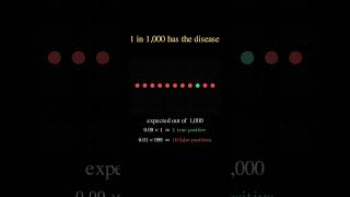
 DeepCamp AI