Deep Learning Crash Course for Beginners
Key Takeaways
Introduces deep learning concepts and terminology for beginners
Full Transcript
You've probably read in the news that deep learning is the secret recipe behind many exciting developments and has made many of our wildest dreams and perhaps also nightmares come true. Who would have thought that Deep Minds Alpha Go could be at least a doll in a board game which boasts of more possible moves than there are atoms in the entire universe. A lot of people including me never saw it coming. It seemed impossible but it's here now. Deep learning is everywhere. It's beating physicians at diagnosing cancer. is responsible for translating web pages in a matter of mere seconds to the autonomous vehicles by Whimo and Tesla. Hi, my name is Jason and welcome to this course in deep learning where you'll learn everything you need to get started with deep learning and Python. How to build remarkable algorithms capable of solving complex problems that weren't possible just a few decades ago. We'll talk about what deep learning is and the difference between artificial intelligence and machine learning. I'll introduce neural networks, what they are, and just how essential they are to deep learning. You're going to learn about how deep learning models train and learn, and the various types of learning associated, supervised, unsupervised, and reinforcement learning. We're going to talk about loss functions, optimizers, the gradient descent algorithm, the different types of neural network architectures, and the various steps involved in deep learning. This entire course is centered on the notion of deep learning. But what is it? Deep learning is a subset of machine learning which in turn is a subset of artificial intelligence which involves more traditional methods to learn representations directly from data. Machine learning involves teaching computers to recognize patterns in data in the same way as our brains do. So as humans, it's easy for us to distinguish between a cat and a dog. But it's much more difficult to teach a machine to do this. And we'll talk more about this later on in this course. Before I do that, I want to give you a sense of the amazing successes of deep learning in the past. In 1997, Gary Kasparov, the most successful champion in the history of chess, lost to IBM's Deep Blue, one of the first computer or artificial systems. It was the first defeat of a reigning world chess champion by a computer. In 2011, IBM's Watson competed in the game show Jeopardy against his champions Brad Roter and Ken Jennings and won the first prize of a million dollars. In 2015, Alph Go, a deep learning computer program created by Google's deep mind division, defeated Lisa Dole, an 18time world champion at Go, a game a Google more times complex than chess. But deep learning can do more than just beat us at board games. It finds applications anywhere from self-driving vehicles to fake news detection to even predicting earthquakes. These were astonishing moments, not only because machines beat humans at their own games, but because of the endless possibilities that they opened up. What followed such events have been a series of striking breakthroughs in artificial intelligence, machine learning, and yes, deep learning. To put it simply, deep learning is a machine learning technique that learns features and tasks directly from data by running inputs through a biologically inspired neuronet network architecture. These neural networks contain a number of hidden layers through which data is processed, allowing for the machine to go deep in its learning, making connections and weighing input for the best results. We'll go over neuronet networks in the next video. So, why deep learning? The problem with traditional machine learning algorithms is that no matter how complex they get, they'll always be machine-like. They need a lot of domain expertise, human intervention, and are only capable of what they designed for. For example, if I show you the image of a face, you will automatically recognize it's a face. But how would a computer know what this is? Well, if we follow traditional machine learning, we have to manually and painstakingly define to a computer what a face is. For example, it has eyes, ears, and a mouth. But now, how do you define an eye or a mouth to a computer? Well, if you look at an eye, the corners are at some angle. They're definitely not 90°. They're definitely not 0°. There some angle in between. So, we could work with that and train our classifier to recognize these kinds of lines in certain orientations. This is complicated. For AI practitioners and the rest of the world, that's where deep learning holds a bit of promise. The key idea in deep learning is that you can learn these [clears throat] features just from raw data. So I can feed a bunch of images of faces to my deep learning algorithm and it's going to develop some kind of hierarchical representation of detecting lines and edges and then using these lines and edges to detect eyes and a mouth and composing it together to ultimately detect the face. As it turns out, the underlying algorithms for training these models have existed for quite a long time. So why is deep learning gaining popularity many decades later? Well, for one, data has become much more pervasive. We're living in the age of big data and these algorithms require massive amounts of data to effectively be implemented. Second, we have hardware and architecture that are capable of handling the vast amounts of data and computational power that these algorithms require. Hardware that simply wasn't available a few decades ago. Third, building and deploying these algorithms or models as they're called is extremely streamlined with the increasing popularity of opensource software like TensorFlow and PyTorch. Deep learning models refer to the training of things called neural networks. Neural networks form the basis of deep learning, a sub field of machine learning where algorithms are inspired by the structure of the human brain. Just like neurons make up the brain, the fundamental building blocks of a neuronet network is also a neuron. Neural networks take in data. They train themselves to recognize patterns in this data and predict outputs for a new set of similar data. In a new network, information propagates through three central components that form the basis of every neuronet network architecture. The input layer, the output layer, and several hidden layers between the two. In the next video, we'll go over the learning process of a neural network. The learning process of a neural network can be broken into two main processes. Forward propagation and back propagation. Forward propagation is the propagation of information from the input layer to the output layer. We can define our input layer as several neurons X1 through XN. These neurons connect to the neurons of the next layer through channels and they are assigned numerical values called weights. The inputs are multiplied to the weights and their sum is sent as input to the neurons in the hidden layer where each neuron in turn is associated to a numerical value called the bias which is then added to the input sum. This weighted sum is then passed through a nonlinear function called the activation function which essentially decides if that particular neuron can contribute to the next layer. In the output layer, it's basically a form of probability. The neuron with the highest value determines what the output finally is. So let's go over a few terms. The weight of a neuron tells us how important the neuron is. The higher the value, the more important it is in the relationship. The bias is like the neuron having an opinion to the relationship. It serves to shift the activation function to the right or to the left. If you have had some experience with high school math, you should know that adding a scalar value to a function shifts the graph either to the left or to the right. And this is exactly what the bias does. It shifts the activation function to the right or to the left. Back propagation is almost like for propagation except in the reverse direction. Information here is passed from the output layer to the hidden layers, not the input layer. But what information gets passed on from the output layer? Isn't the output layer supposed to be the final layer where we get the final output? Well, yes, but no. Back propagation is the reason why neural networks are so powerful. It is the reason why neural networks can learn by themselves. In the last step of all propagation, a new network spits out a prediction. This prediction could have two possibilities either right or wrong. In bad propagation, the new network evaluates its own performance and checks if it is right or wrong. If it is wrong, the network uses something called a loss function to quantify the deviation from the expected output. And it is this information that's sent back to the hidden layers for the weights and biases to be adjusted so that the network's accuracy level increases. Let's visualize the training process with a real example. Let's suppose we have a data set. This data set gives us the weight of a vehicle and the number of goods carried by that vehicle and also tells us if those vehicles are cars or trucks. We want to go through this data, train a new networks to predict cars or trucks based on their weights and goods. To start off, let's initialize the neural network by giving it random weights and biases. These can be anything. We really don't care what these values are as long as they're there. In the first entry of a data set, we have vehicle weight equal to a value which in this case is 15 and goods as two. According to this, it's a car. We now start moving these input dimensions through the newer network. So basically what we want to do is take both the inputs, multiply them by their weight, and add a bias. And this is where the magic happens. We run this weighted sum through an activation function. Okay. Now let's say that the output of this activation function is 0001. This again is multiplied by the weights and added to the bias. And finally in the output layer we have a guess. Now according to this neuronet network the type of vehicle with weight 15 and goods 2 has a greater probability of being a truck. Of course this is not true and a neuronet network knows this. So we use back propagation. We're going to quantify the difference between the expected result and the predicted output using a loss function. In back propagation, we're going to go backwards and adjust our initial weights and biases. Remember that during the initialization of the new network, we chose completely random weight and biases. Well, during back propagation, these values will be adjusted to better fit the prediction model. Okay, so that was one iteration through the first piece of the data set. In the second entry, we have vehicle weight 34 and goods 67. We're going to use the same process as before. Multiply the input with the weight and add a bias. Pass as a result into an activation function and repeat till the output layer. Check the error difference and employ back propagation to adjust the weights in the biases. Your new network will continue doing this repeated process of for propagation, calculating the error and then back propagation for as many entries there are in this data set. [snorts] The more data you give the new network, the better it will be at predicting the right output. But there's a trade-off because too much data and you'll end up with a problem like overfitting which I'll discuss later on in this course. But that's essentially how new network works. You feed input, the network initializes with random weights and biases that are adjusted each time during back propagation until the network's gone through all your data and is now able to make predictions. This learning algorithm can be summarized as follows. First, we initialize the network with random values for the network's parameters or the weights and the biases. We take a set of input data and pass them through the network. We compare these predictions obtained with the values of the expected labels and calculate the loss using loss function. We perform back propagation in order to propagate this loss to each and every weight and bias. We use this propagated information to update the weights and biases of neuronet network with the gradient descent algorithm in such a way that the total loss is reduced and a better model is obtained. The last step is continue iterating the previous steps until we consider that we have a good enough model. In this section, we're going to talk about the most common terminologies used in deep learning today. Let's start off with the activation function. The activation function serves to introduce something called nonlinearity into the network and also decides whether a particular neuron can contribute to the next layer. But how do you decide if the neuron can fire or activate? Well, we had a couple of ideas which led to the creation of different activation functions. The first idea we had is how about we activate the neuron if it is above a certain value or threshold. If it is less than this threshold, don't activate it. Activation function A is equal to activated if Y is greater than some threshold. Else it's not. This is essentially a step function. Its output is one or activated when value is greater than zero. Its output is activated when value is greater than some threshold and outputs not activated otherwise. Great. So this makes an activation function for a neuron. No confusions. Life is perfect. Except there are some drawbacks with this. To understand it better, think about the following. Think about a case where you want to classify multiple such neurons into classes. Say class one, class 2, class 3, etc. What will happen if more than one neuron is activated? All these neurons will output a one. Well, how do you decide now? How do you decide which class it belongs to? It's complicated, right? You would want the network to activate only one neuron and the other should be zero. only then you would be able to see it was classified properly. In real practice, however, it is harder to train and converge this way. It would be better if the activation was not binary and instead some probable value like 75% activated or 16% activated. There's a 75% chance that it belongs to class 2, etc. Then, if more than one neuron activates, you could find which neuron fires based on which has the highest probability. Okay, maybe you'll ask yourself, I want something to give me a more analog value rather than just saying activated or not activated, something other than in binary. And maybe you would have thought about a linear function, a straight line function where the activation is proportional to the input by a value called the slope of the line. This way, it gives us a range of activations. So, it isn't binary activation. [clears throat] We can definitely connect a few neurons together and if more than one fires, we could take the maximum value and decide based on that. So that is okay too. And what is the problem with this? Well, if you are familiar with gradient descent, which I'll come to in just a bit, you'll notice that the derivative of a linear function is a constant. Makes sense because the slope isn't changing at any point. For a function f ofx is equal to mx plus c, the derivative is m. This means that the gradient has no relationship whatsoever with X. This also means that during back propagation, the adjustments made to the weights and the biases aren't dependent on X at all. And this is not a good thing. Additionally, think about if you have connected layers. No matter how many layers you have, if all of them are linear in nature, the activation function of the final layer is nothing but just a linear function of the input of the first layer. Pause for a bit and think about it. This means that the entire new network of dozens of layers can be replaced by a single layer. Remember, a combination of linear functions in a linear manner is still another linear function. And this is terrible because we've just lost the ability to stack layers this way. No matter how much we stack, the whole network is still equivalent to a single layer with single activation. Next, we have a sigmoid function. And if you've ever watched the video on activation functions, this is the kind of function used in the examples. A sigmoid function is defined as a of x is equal to 1 / 1 + ex. Well, this looks smooth and kind of like a step function. What are its benefits? Think about it for a moment. Well, first things first, it is nonlinear in nature. Combinations of this function are also nonlinear. Great. So now we can stack layers. What about non-binary activations? Yes, that too. This function outputs an analog activation unlike the step function and also has a smooth gradient. An advantage of this activation function is that unlike the linear function, the output of this function is going to be in the range 0 to 1 inclusive compared to the negative infinity to infinity of the latter. So we have our activations bound in a range and this won't blow up the activations. And this is great and sigmoid functions are one of the most widely used activation functions today. But life isn't always rosy and sigmoids too tend to have the share of disadvantages. If you look closely between x= to -2 and x= 2, the y values are very steep. Any small changes in values of x in that region will cause values of y to change drastically. Also towards either end of the function, the y values tend to respond very or less to changes in x. The gradient at those regions is going to be really really small, almost zero. And it gives rise to the vanishing gradient problem which just says that if the input of the activation function is either large or small the sigmoid is going to squish that down to a value between zero and one and the gradient of this function becomes really small and you'll see why when we talk about gradient sent this is a huge problem. Another activation function that is used is the tanh function. This looks very similar to sigmoid. In fact, mathematically, this is what's known as a shifted sigmoid function. Okay. So, like the sigmoid, it has characteristics that we discussed above. It is nonlinear in nature. So, we can stack layers. It is bound to a range from -1 to 1. So, there's no worrying about the activations blowing up. The derivative of the tanh function, however, is steeper than that of the sigmoid. So, deciding between the sigmoid and the tanh will really depend on your requirement of the gradient strength. Like sigmoid, tanh is also a very popular and widely used activation function. And yes, like the sigmoid, tanh does have a vanishing gradient problem. The rectified linear unit or the value function is defined as if x is equal to the max from 0 to x. At first look, this would look like a linear function, right? The graph is linear in the positive axis. Let me tell you, relu is in fact nonlinear in nature and combinations of relu are also nonlinear. Great. So this means that we can stack layers. However, unlike the previous two functions that we discussed, it is not bounded. The range of the relu is from 0 to infinity. This means there is a chance of blowing up the activation. Another point that I would like to discuss here is sparity of an activation. Imagine a big neuron network with lots of neurons. Using a sigmoid or a tan will cause almost all the neurons to fire in an analog way. This means that almost all activations will be processed to describe the network's output. In other words, the activation would be dense and this is costly. Ideally, we want only a few neurons in the network to activate and thereby making the activation sparse and efficient. Here's where the relu comes in. Imagine a network with randomly initialized weights and almost 50% of the network yields zero activation. Because of the characteristic of ReLU, it outputs zero for negative values of X. This means that only 50% of the neurons fire sparse activation making the network lighter. But when life gives you an apple, it comes with a little worm inside. Because of that horizontal line in relu for negative values of X, the gradient is zero in that region. Which means that during back propagation, the weights will not get adjusted during descent. This means that those neurons which go into that state will stop responding to variations in the error simply because the gradient is zero. Nothing changes. This is called the dying rel problem. This problem can cause several neurons to just die and not respond. Thus making a substantial part of the network passive rather than what we want active. There are workarounds for this. One way especially is to simply make the horizontal line into a nonh horizontal component by adding a slope. Usually the slope is around 0001 and this this new version of the relu is called the leaky relu. The main idea is that the gradient should never be zero. One major advantage of the relu is the fact that it's less computationally expensive than functions like tanhage and sigmoid because it involves simpler mathematical operations. This is a really good point to consider when you were designing your own deep neural networks. Great. So now the question is which activation function to use? Because of the advantages that rel offers, does this mean that you should use rel for everything you do? Or could you consider sigmoid and 10h? Well, both. When you know the function that you're trying to approximate has certain characteristics, you should choose an activation function but which will approximate the function faster leading to faster training processes. For example, a sigmoid function works well for binary classification problems because approximating our classifier functions as combinations of the sigmoid is easier than maybe the relu. This will lead to faster training processes and larger convergence. You can use your own custom functions too. If you don't know the nature of the function you're trying to learn, I would suggest you start with relu and then work backwards from there. Before we move on to the next section, I want to talk about why we use nonlinear activation functions as opposed to linear ones. If you recall in my definition of activation functions, I mentioned that activation functions serve to introduce something called nonlinearity in the network. For all intents and purposes, introducing nonlinearity simply means that your activation function must be nonlinear. That [snorts] is not a straight line. Mathematically linear functions are polomials of degree 1 that when graphed in the xy plane are straight lines inclined to the x-axis at a certain value. We call this the slope of the line. Nonlinear functions are polomials of degree greater than one. And when graphed they don't form straight lines rather than more curved. If we use linear activation functions to model our data, then no matter how many hidden layers a network has, it will always become equivalent to having a single layer network. And in deep learning, we want to be able to model every type of data without being restricted as would be the case should we use linear functions. We've discussed previously in the learning process of neuronet networks that we start off with random weights and biases. The neural network makes a prediction. This prediction is compared against the expected output and the weights and biases adjusted accordingly. Well, loss functions are the reason that we're able to calculate that difference. Really simply, a loss function is a way to quantify the deviation of the predicted output by the neural network to the expected output. It's as simple as that. Nothing more, nothing less. There are plenty of loss functions out there. For example, under regression, we have squared error loss, absolute error loss, and hub loss. In binary classification, we have binary cross entropy and hinge loss. In multiclass classification problems, we have the multiclass cross entropy and the callback liel divergence loss and so on. The choice of the best function really depends on what kind of project you're working on. Different projects require different loss functions. Now, I don't want to talk any further on loss functions right now. We'll do this under the optimization section because that's really where loss functions are utilized. In the previous section, we dealt with loss functions which are mathematical ways of measuring how wrong predictions made by new network are. During the training process, we tweak and change the parameters or the weights of the model to try and minimize that loss function and make our predictions as correct and optimized as possible. But how exactly do you do that? How do you change the parameters of your model by how much and when? We have the ingredients. How do we make the cake? This is where optimizers come in. They tie together the loss function and the model parameters or the weight and biases by updating the network in response to the output of the loss function. In simpler terms, optimizers shape and mold your model into more accurate models by adjusting the weights and the biases. The loss function is its guide. It tells the optimizer whether it's moving in the right or the wrong direction. To understand this better, imagine that you have just scaled Mount Everest and now you decide to descend the mountain blindfolded. It's impossible to know which direction to go in. You could either go up, which is away from your goal, or go down, which is towards your goal. But to begin, you would start taking steps. Using your feet, you'll be able to gauge whether you're going up or down. In this analogy, you resemble the neural network. going down your goal is trying to minimize the error and your feet are resemblant of the loss functions. They measure whether you're going in the right way or the wrong way. Similarly, it's impossible to know what your model's weights should be right from the start. But with some trial and error based on the loss function, you could end up getting there eventually. We now come to gradient descent, often called the granddaddy of optimizers. Gradient descent is an iterative algorithm that starts off at a random point in the loss function and travels down its slope in steps until it reaches the lowest point or the minimum of the function. It is the most popular optimizer we use nowadays. It's fast, robust, and flexible. And here's how it works. First, we calculated what a small change in each individual weight would do to the loss function. We adjust each individual weight based on its gradient. that is take a small step in the determined direction. The last step is to repeat the first and the second step until the loss function gets as low as possible. I want to talk about this notion of a gradient. The gradient of a function is the vector of the partial derivatives with respect to all independent variables. The gradient always points in the direction of the steepest increase in the function. Suppose we have a graph like so with loss on the y-axis and the value of the weight on the x-axis. We have a little data point here that corresponds to the randomly initialized weight. To minimize its loss, that is to get this data point to the minimum of the function, we need to take the negative gradient since we want to find the steepest decrease in the function. This process happens iteratively till the loss is as minimized as possible. And that's gradient descent in a nutshell. When dealing with highdimensional data sets, that is lots of variables, it's possible you'll find yourself in an area where it seems like you've reached the lowest possible value for your loss function, but in reality, it's just a local minimum. To avoid getting stuck in a local minima, we make sure we use the proper learning rate. Changing our weights too fast by adding or subtracting too much, that is taking steps that are too large or too small, can hinder your ability to minimize the loss function. We don't want to make a jump so large that we skip over the optimal value for a given weight. To make sure this doesn't happen, we use a variable called the learning rate. This thing is usually just a small number like 0.1 that we multiply the gradients by to scale them. This ensures that any changes we make to our weight are pretty small. In math talk, taking steps that are too large can mean that the algorithm will never converge to an optimum. At the same time, we don't want to take steps that are too small because then we might never end up with the right values for our weights. In math talk, steps that are too small might lead to our optimizer converging on a local minimum for the loss function, but never the absolute minimum. For a simple summary, just remember that the learning rate ensures that we change our weight at the right pace. Not making any changes that are too big or too small. Instead of calculating the gradients for all your training examples on every pass of the gradient descent, it's sometimes more efficient to only use a subset of the training examples each time. Stoastic gradient descent is an implementation that either uses batches of examples at a time or random examples on each pass. Stochcastic gradient descent uses the concept of momentum. Momentum accumulates gradients of the past steps to dictate what might happen in the next steps. Also, because we don't include the entire training set, SGD is less computationally expensive. It's difficult to overstate how popular gradient descent really is. Back propagation is basically gradient descent implemented on a network. There are other types of optimizers based on gradient descent that are used today. Adagrad adapts the learning rate specifically to individual features. That means that some of the weights in your data set will have different learning rates than others. This works really well for sparse data sets where a lot of input examples are missing. Adrad has a major issue though. The adaptive learning rate tends to get really really small over time. RMS prop is a special version of Adrad developed by Professor Jeffrey Hinton. Instead of letting all the gradients accumulate for momentum, it accumulates gradients in a fixed window. RMS prop is similar to add a prop which is another optimizer that seeks to solve some of the issues that adrad leaves open. Atom stands for adaptive moment estimation and is another way of using past gradients to calculate the current gradient. Adam also utilizes the concept of momentum, which is basically our way of telling the new network whether we want past changes to affect the new change by adding fractions of the previous gradients to the current one. This optimizer has become pretty widespread and is practically accepted for use in training new networks. It's easy to get lost in the complexity of some of these new optimizers. Just remember that they all have the same goal, minimizing the loss function, and trial and error will get you there. You may have heard me referring to the words parameters quite a bit and often this word is confused with the term hyperparameters. In this video, I'm going to outline the basic difference between the two. A model parameter is a variable that is internal to the neural network and whose values can be estimated from the data itself. They are required by the model when making predictions. These values define the scale of the model on your problem. They can be estimated directly from the data and are often not manually set by the practitioner. And often times when you save your model, you are essentially saving your model's parameters. Parameters are key to machine learning algorithms. And examples of these include the weights and the biases. A hyperparameter is a configuration that is external to the model and whose value cannot be estimated from data. There's no way that we can find the best value for a model hyperparameter on a given problem. We may use rules of thumb, copy values used in other problems or search for the best value by trial and error. When a machine learning algorithm is tuned for a specific problem, such as when you're using grid search or random search, then you are in fact tuning the hyperparameters of the model in order to discover the parameters that result in more skillful predictions. Model hyperparameters are often referred to as parameters which can make things confusing. So a good rule of thumb to overcome this confusion is as follows. If you have to specify a parameter manually, then it is probably a hyperparameter. parameters are inherent to the model itself. Some examples of hyperparameters include the learning rate for training a new network, the C and sigma hyperparameters for sport vector machines and the K and K nearest neuros neighbors. We need terminologies like epochs, batch size, and iterations only when the data is too big, which happens all the time in machine learning and when we can't pass all this data to the computer at once. So to overcome this problem, we need to divide the data set into smaller chunks, give it to our computer one by one, and update the weights of the new network at the end of every step to fit it into the data given. One epoch is when an entire data set is passed forward and backward through the network once. In a majority of deep learning models, we use more than one epoch. I know it does make sense in the beginning. Why do we need to pass the entire data set many times through the same neural network? Passing the entire data set through the network only once is trying to read the entire lyrics of a song once. You won't be able to remember the entire song immediately. You'd have to reread the lyrics a couple more times before you can say you know the song by memory. The same is true with the neuronet network. We pass the data set multiple times through the neuronet network so it's able to generalize better. Gradient descent is an iterative process. And updating the parameters and back propagation in a single pass or one epoch is not enough. As the number of epochs increases, the more the parameters are adjusted, leading to a better performing model. But too many epochs could spell disaster. Indeed, is something called overfitting, where a model has essentially memorized the patterns in the training data and performs terribly on data it's never seen before. So what is the right number of epochs? Unfortunately, there is no right answer. The answer is different for different data sets. Sometimes your data set can include millions of examples. Passing this entire data set at once becomes extremely difficult. So what we do instead is divide the data set into a number of batches rather than passing the entire data set once. The total number of training examples present in a single batch is called a batch size. Iterations is the number of batches needed to complete one epoch. Note the number of batches is equal to the number of iterations for one epoch. Let's say that we have a data set of 34,000 training examples. If we divide the data set into batches of 500, then it will take 68 iterations to complete one epoch. Well, I hope that gives you some kind of sense about the very basic terminologies used in deep learning. Before we move on, I do want to mention this and you'll see this a lot in deep learning. You'll often have a bunch of different choices to make. How many hidden layers should I choose? Or which activation function must I use and where? And to be honest, there are no clear-cut guidelines as to what your choice should always be. That's the fun part about deep learning. It's extremely difficult to know in the beginning what's the right combination to use for your project. What works for me might not work for you. And a suggestion from my end would be that you dabble along with the material shown. Try various combinations and see what works for you best. Ultimately, that's a learning process, pun intended. Throughout this course, I'll give you quite a bit of intuition as to what's popular so that when it comes to building a deep learning project, you won't find yourself lost. In this section, we're going to talk about the different types of learning, which are machine learning concepts, but are extended to deep learning as well. In this course, we'll go over supervised learning, unsupervised learning, and reinforcement learning. Supervised learning is the most common subbranch of machine learning today. Typically, if you're new to machine learning, your journey will begin with supervised learning algorithms. Let's explore what these are. Supervised machine learning algorithms are designed to learn by example. The name supervised learning originates from the idea that training this type of algorithm is almost like there's a human supervising the whole process. In supervised learning, we train our models on well-labeled data. Each example is a pair consisting of an input object, which is typically a vector, and a desired output value, also called a supervisory signal. During training, a supervised learning algorithm will search for patterns in the data that correlate with the desired outputs. After training, it will take in new unseen inputs and will determine which label the new inputs will be classified as based on prior training data. The objective of a supervised learning model is to predict the correct label for newly presented input data. At its most basic form, a supervised learning algorithm can simply be written as y is equal fx where y is the predicted output that is determined by a mapping function that assigns a class to an input value x. The function used to connect input features to a predicted output is created by the machine learning model during training. Supervised learning can be split into two subcategories classification and regression. During training, a classification algorithm will be given data points with an assigned category. The job of a classification algorithm is then to take this input value and assign to a class of category that it fits into based on the training data provided. The most common example of classification is determining if an email is spam or not. With two classes to choose from, spam or not spam, this problem is called a binary classification problem. The algorithm will be given training data with emails that are both spam and not spam and the model will find the features within the data that correlate to either class and create a mapping function. Then when provided with an unseen email, the model will use this function to determine whether or not the email is spam. An example of a classification problem would be the emnest handwritten digits data set where the inputs are images of handwritten digits or pixel data and the output is a class label for what digit the image represents that is numbers 0 to 9. There are numerous algorithms to solve classification problems each which depends on the data and the situation. Here are a few popular classification algorithms. linear classifiers, support vector machines, decision trees, k nearest neighbors, and random forest. Regression is a predictive statistical process where the model attempts to find the important relationship between dependent and independent variables. The goal of a regression algorithm is to predict a continuous number such as sales, income, and tax codes. The equation for a basic linear regression can be written as follows. Where x of i represents the features of the data and w of i and b are parameters which are developed during training. For simple linear regression models with only one feature in the data, the formula looks like this where w is the slope, x is the single feature, and b is the y intercept. Familiar? For simple regression problems such as this, the model's predictions are represented by the line of best fit. For models using two features, a plane is used. And for models with more than two features, a hyper plane is used. Imagine we want to determine a student's test grade based on how many hours they studied the week of the test. Let's say the plot data with line of best fit looks like this. There is a clear positive correlation between R studied, the independent variable, and the students final test scores, the dependent variable. A line of best fit can be drawn through the data points to show the model's predictions when given a new input. Say we wanted to know how well a student would do with 5 hours of studying. We can use the line of best fit to predict the test score based on other students performances. Another example of regression problem would be the Boston house prices data set where the input of variables that describe a neighborhood and the output is a house price in dollars. There are many different types of regression algorithms. Three most common are linear regression, lasser regression and multivaried regression. Supervised learning finds applications in classification and regression problems like bioinformatics such as fingerprint, iris and face recognition in smartphones, object recognition, spam detection and speech recognition. Unsupervised learning is a branch of machine learning that is used to manifest underlying patterns in data and is often used in exploratory data analysis. Unlike supervised learning, unsupervised learning does not use label data, but instead focuses on the data's features. Label training data has a corresponding output for each input. The goal of an unsupervised learning algorithm is to analyze data and find important features in that data. Unsupervised learning will often find subgroups or hidden patterns within the data set that a human observer might not pick up on. And this is extremely useful as we'll soon find out. Unsupervised learning can be of two types, clustering and association. Clustering is the simplest and among the most common applications of unsupervised learning. It is the process of grouping the given data into different clusters or groups. Clusters will contain data points that are as similar as possible to each other and as dissimilar as possible to data points in other clusters. Clustering helps find underlying patterns within the data that may not be noticeable to a human observer. It can be broken down into partitional clustering and hierarchical clustering. Partitional clustering refers to a set of clustering algorithms where each data point in a data set can belong to only one cluster. Hierarchical clustering finds clusters by a system of hierarchies. Every data point can belong to multiple clusters. Some clusters will contain smaller clusters within it. This hierarchy system can be organized as a tree diagram. Some of the more commonly used clustering algorithms are the K means expectation maximization and the hierarchical cluster analysis or the ACA. Association on the other hand attempts to find relationships between different entities. The classic example of association rules is market basket analysis. This means using a database of transactions in a supermarket to find items that are frequently bought together. For example, a person who buys potatoes and burgers usually buys beer. For example, a person who buys tomatoes and pizza cheese might want to bring pizza bread and so on. Unsupervised Lonely finds applications almost everywhere. For example, Airbnb, which helps host stays and experiences and connect people all over the world. This application uses unsupervised learning algorithms where a potential client queries their requirements and Airbnb learns these patterns and recommend stays and experiences which fall under the same group of cluster. Example, a person looking for houses in San Francisco might not be interested in finding houses in Boston. Amazon also uses unsupervised learning to learn the customers purchases and recommend products which are frequently bought together which is an example of association rule mining. Credit card fraud detection is another unsupervised learning algorithm that learns the various patterns of a user and and their usage of a credit card. If the card is used in parts that do not match the behavior, an alarm is generated which could possibly be marked as fraud. And in some cases, your bank might call you to confirm whether it was you using the card or not. Reinforcement learning is a type of machine learning technique that enables an agent to learn in an interactive environment by trial and error using feedback from its own actions and experiences. Like supervised learning, it uses mapping between the input and the output. But unlike supervised learning where feedback provided to the agent is a correct set of actions for performing a task, reinforcement learning uses rewards and punishments as signals for positive and negative behavior. When you compared with unsupervised learning, reinforcement learning is different in terms of its goals. While the goal in unsupervised learning is to find similarities and differences between data points, in reinforcement learning, the goal is to find a suitable action model that would maximize the total cumulative reward of the agent. Reinforcement learning refers to goal oriented algorithms which learn how to attain a complex objective or goal or how to maximize along a particular dimension over many steps. For example, they can maximize the points one in a game over many moves. Reinforcement learning algorithms can start from a blank slate and under the right conditions achieve superhuman performance like a pet incentivized by scolding and treats. These algorithms are penalized when they make the wrong decisions and rewarded when they make the right ones. This is reinforcement. Reinforcement learning is usually modeled as a mark of decision process. Although other frameworks like Q-learning are used. Some key terms that describe the elements of a reinforcement learning problem are the environment which is the physical world in which the agent operates. The state represents the current situation of the agent. Reward is a feedback received from the environment. Policy sometimes is the method to map the agent state to the agents actions. And finally, value is a future reward that an agent will receive by taking an action in a particular state. A reinforcement learning problem can be best explained through games. Let's take the game of Pac-Man where the goal of the agent or Pac-Man is to eat the food in the grid while avoiding the ghost on its way. The grid world is the interactive environment for the agent. Pac-Man receives a reward for eating food and punishment if it gets killed by the ghost. That is, it loses the game. The states are the location of Pac-Man in the grid world. And the total cumulative reward is Pac-Man winning the game. Reinforcement learning finds applications in robotics, business strategy planning, traffic light control, web system configuration, and aircraft and robot motion control. A central problem in deep learning is how to make an algorithm that will perform well not just on training data, but also on new inputs. One of the most common challenges you'll face when training models is a problem of overfitting. a situation where your model performs exceptionally well on training data but not on testing data. Say I have a data set graphed on the XY plane like so. Now I want to construct a model that would best fit the data set. What I could do is draw a line of some random slope and intercept. Now evidently this isn't the best model and in fact this is called underfitting because it doesn't fit the model well. In fact it underestimates the data set. Instead, what we could do is draw a line that looks something like this. Now, this really fits our model the best. But this is overfitting. Remember that while training, we show our network some training data. And once that's done, we'd expect it to be almost close to perfect. The problem with this graph is that although it is probably the best line of fit for this graph, it is the best line of fit only if you're considering your trading data. What your network has done in this graph is memorize the patterns between the training data and won't give accurate predictions at all on data it's never seen before. And this makes sense because instead of memorizing patterns generally to perform well on both training as well as new testing data, a network in fact has memorized the patterns only on the training data. So it obviously won't perform well on new data it's never seen before. This is the problem of overfitting. It fitted too much. And by the way, this would be the more accurate kind of fitting. It's not perfect, but it'll do well on both training as well as new testing data with sizable accuracy. There are a couple of ways to tackle overfitting. The most interesting type of regularization is dropout. It produces very good results and is consequently the most frequently used regularization technique in the field of deep learning. To understand dropout, let's say that we have a neural network with two hidden layers. What dropout does is that at every iteration, it randomly selects some nodes and removes them along with their incoming and outgoing connections as shown. So each iteration has a different set of nodes and this results in a different set of outputs. So why do these models perform better? These models usually perform better than a single model as they capture more randomness and memorizes less of the training data and hence will be focused generalized better and build a more robust predictive model. Sometimes the best way to make a deep learning model generalize better is to train it on more data. In practice, the amount of data we have is limited. And one way to get around this problem is to create fake data and add it to the training set. For some deep learning tasks, it is reasonably straightforward to create new fake data. This approach is easiest for classification. A classifier needs to take complicated highdimensional input X and summarize it with the category identity Y. This means that the main task facing a classifier is to be invariant to a wide variety of transformations. We can generate new XY pairs easily just by applying transformations on the XY input in our training set. Data set augmentation has been a particularly effective technique for a specific classification problem. Object recognition images are highdimensional and include an enormous range of factors of variation, many of which can easily be simulated. Operations like translating the training images a few pixels in each direction can often greatly improve generalization. Many other operations such as rotating the image or scaling the image have also proved quite effective. You must be careful not to apply transformations that would change the correct class. For example, in optical character recognition tasks that require recognizing the difference between a B and a D and the difference between a six and a nine. Horizontal flips and 180 degree rotations are not appropriate ways of augmenting data sets with these tasks. When training large models with sufficient representational capacity to overfitit the task, we often observe that the training error decreases steadily over time, but the error validation set begins to rise again. This means we can obtain a model with better validation set error and thus hopefully better test set error by stopping training at the point where the error in the validation set starts to increase. This strategy is known as early stopping. It is probably the most commonly used form of regularization in deep learning today. Its popularity is due to both its effectiveness and its simplicity. In this section, I'm going to introduce the three most common types of neural network architectures today. Fully connected V4 neural networks, recurrent neural networks, and convolutional neural networks. The first type of neural network architecture we're going to discuss is a fully connected feed forward neural network. By fully connected I mean that each neuron in the preceding layer is connected to every neuron in the subsequent layer without any connection backwards. There are no cycles or loops in the connections in the network. As I mentioned previously, each neuron in a neuronet network contains an activation function that changes the output of a neuron when given its input. There are several types of activation functions that can change this input to output relationship to make a neuron behave in a variety of ways. Some of the most well-known activation functions are the linear function which is a straight line that essentially multiplies the input by a constant value, the sigmoid function that ranges from 0 to 1, the hyperbolic tangent or the tangent function ranging from -1 to positive 1, and the rectified linear unit or the rel function which is a peace-wise function that outputs a zero if the input is less than a certain value or a linear multiple if the input is greater than a certain value. Each type of activation function has its pros and cons. So we use them in various layers in the deep neural network based on the problem each is designed to solve. In addition, the last three activation functions we refer to as nonlinear functions because the output is not a linear multiple of the input. Nonlinearity is what allows deep neuronet networks to model complex functions. Using everything we've learned so far, we can create a wide variety of fully connected feed forward neuronet networks. We can create networks with various inputs, various outputs, various hidden layers, neurons per hidden layer, and a variety of activation functions. These numerous combinations allow us to create a variety of powerful deep neural networks that can solve a wide array of problems. The more neurons we add to each hidden layer, the wider the network becomes. In addition, the more hidden layers we add, the deeper the network becomes. However, each neuron we add increases the complexity and thus the computational resource necessary to train a neural network increases. This increase in complexity isn't linear in the number of neurons we add. So, it leads to an explosion in complexity and training time for large neural networks. That's a trade-off you need to consider when you are building deep neural networks. All the neural networks we've discussed so far are known as feed forward neural networks. They take in a fixed-sized input and give you a fixed size output. That's all it does. And that's what we expect neural networks to do. Take in an input and give a sizable output. But as it turns out, these plain or vanilla neural networks aren't able to model every single problem that we have today. To better understand this, use this analogy. Suppose I show you the picture of a ball, a round spherical ball that was moving in space in some direction. I've just taken a photo of the ball or a snapshot of the ball at some time t. Now, I want you to predict the next position of the ball in say 2 or 3 seconds. You're probably not going to give me an accurate answer. Now, let's look at another example. Suppose I walk up to you and say the word dog. You will never understand my statement because, well, it doesn't make sense. There are trillion combinations solely using the word dog. And among these trillion combinations, I'm expecting you to now guess what I'm trying to tell you. What these two examples have in common is that it doesn't make sense. It doesn't. In the first case, I'm expecting you to predict the next position in time. And in the second, I'm expecting you to understand what I mean by dog. These two examples cannot be understood and interpreted unless some information about the past was supplied. Now, in the first example, if I give you the previous position states of the ball and now ask you to predict the future trajectory of the ball, you're going to be able to do this accurately. And in the second case, if I give you a full sentence saying, I have a dog. This makes sense because now you understand that out of the trillion possible combinations involving a dog, my original intent was for you to understand that I have a dog. Why did I give you this example? How does this apply to neural networks? In the introduction, I said vanilla neuronet networks can't model every single situation or problem that we have. And the biggest problem, it turns out, is that plain vanilla feed forward neuronet networks cannot model sequential data. Sequential data is data in a sequence. For example, a sentence is a sequence of words. A ball moving in space is a sequence of all its position states. In the sentence that I'd shown you, you understood each word based off your understanding of the previous words. This is called sequential memory. You were able to understand a data point in a sequence by your memory of the previous data point in that sequence. Traditional neuronet networks can't do this and it seems like a major shortcoming. One of the disadvantages of modeling sequences with traditional neuronet networks is the fact that they don't share parameters across time. Let us take for example these two sentences. On Tuesday it was raining and it was raining on Tuesday. These sentences mean the same thing although the details are in different parts of the sequence. Actually when we feed these sentences into a feed for neuronet network for a prediction task the model will assign different weights to on Tuesday and it was raining at each moment in time. things we learn about the sequence won't transfer if they appear at different points in the sequence. Sharing parameters gives the network the ability to look for a given feature everywhere in the sequence rather than just in a certain area. Thus, to model sequences, we need a specific learning framework able to deal with variable length sequences, maintain sequence order, and to keep track of long-term dependencies rather than cutting input data too short. and finally to share parameters across the sequence so as to not relearn things. And that's where recurrent neural networks come in. RNNs are a type of neural network architecture that use something called a feedback loop in the hidden layer. Unlike feed forward neural networks, the recurrent neural network or RNN can operate effectively on sequences of data with variable input length. This is how an RNN is usually represented. This little loop here is called the feedback loop. Sometimes you may find the RNN's depicted over time like this. The first path represents the network in the first time step. The hidden node H1 uses the input X1 to produce output Y1. This is exactly what we've seen with basic feed for new networks. However, at the second time step, the hidden node at the current time step h2 uses both the new input x2 as well as the state from the previous time step h1 as input to make new predictions. This means that a current neural network uses knowledge of its previous states as input for its current prediction. And we can repeat this process for an arbitrary number of steps allowing for the network to propagate information by its hidden state throughout time. This is almost like giving a neural network a short-term memory. They have this abstract concept of sequential memory. And because of this, we're able to model certain areas of data, sequential data, that standalone new networks aren't able to model. Recurrent neural networks remember their past and their decisions are influenced by what it has learned from the past. Basic feed forward networks remember things too, but they remember things they learned during training. For example, an image classifier learns what a three looks like during training and then uses that knowledge to classify things in production. So how do we train an RNN? Well, it is almost the same as training a basic fully connected fever network except that the back propagation algorithm is applied for every sequence data point rather than the entire sequence. This algorithm is sometimes called the back propagation through time algorithm or the BTT algorithm. To really understand how this works, imagine we're creating a recurrent neural network to predict the next letter a person is likely to type based on the previous letters they've already typed. The letter that a user just typed is quite important to predicting the new letter. However, all the previous letters are also very important to this prediction as well. At the first time step, say the user typed the letter F. So a network might predict that the next letter is an E based on all of the previous training examples that included the word FE. At the next time step, the user types the letter R. So a network uses both the new letter R plus the state of the first hidden neuron in order to compute the next prediction L. The network predicts this because of the high frequency of occurrences in the word feel in our training data set. Adding the letter A might predict the letter T. Adding an N would predict the letter K which would match the word our user intended to type which is frank. There however is an issue with RNN's known as short-term memory. Short-term memory is caused by the infamous vanishing and exploding gradient problems. As the RNN processes more words, it has trouble retaining information from previous steps. Kind of like our memory. If you're given a long sequence of numbers like pi and you tried reading them out, you're probably going to forget the initial few digits, right? Short-term memory and the vanishing gradient is due to the nature of back propagation, the algorithm used to train and optimize neural networks. After the forward propagation or the pass, the network compares this prediction to the ground truth using a loss function which outputs an error value, an estimate of how poorly the network is performing. The network uses that error value to perform back propagation which calculates a gradient for each node in the network. The gradient is a value used to adjust the network's internal weights, allowing for the network to learn. The bigger the gradient, the bigger the adjustments are and vice versa. Here's where the problem lies. When performing back propagation, each node in a layer calculates its gradient with respect to the effects of the gradient in the layer before it. So if the adjustment to the layers before it is small, then the adjustments to the current layer will be even smaller and this causes gradients to exponentially shrink as it back propagates down. The earlier layers fail to do any learning as the internal weights are barely being adjusted due to extremely small gradients and that is the vanishing gradient problem. Let's see how this applies to recover new networks. You can think of each time step in a recurrent new network as a layer. To train a recurren new network, you use an application of back propagation called back propagation through time. The gradient values will exponentially shrink as the back propagates through each time step. Again, the gradient is used to make adjustments in the new network weights, thus allowing it to learn. Small gradients means small adjustments, and this causes the early layers not to learn. Because of the vanishing gradients, the RNN doesn't learn the long range dependencies across time steps. This means that in a sequence it was raining on Tuesday, there is a possibility that the words it and was are not considered when trying to predict the user's intention. The network then has to make the best guess with on Tuesday and that's pretty ambiguous and would be difficult even for a human. So not being able to learn on earlier time steps causes the network to have a short-term memory. We can combat the short-term memory of an RNN by using two variants of recurrent neuronet networks. Gated RNNs and long short-term memory RNNs, also known as LSTMs. Both these variants function just like RNN's, but they're capable of learning long-term dependencies using mechanisms called gates. These gates are different tensor operations that learn information that can learn what information to add or remove to the hidden state of the feedback loop. The main difference between a gated RNN and an LSCM is that the gated RNN has two gates to control its memory. An update gate and a reset gate, while an LSM has three gates, an input gate, an output gate, and a forget gate. RNN's work well for applications that involve sequences of data that change over time. These applications include natural language processing, sentiment classification, DNA sequence classification, speech recognition, and language translation. A convolutional neuronet network or CNN for short is a type of deep neuronet network architecture designed for specific tasks like image classification. CNN's were inspired by the organization of neurons in the visual cortex of the animal brain. As a result, they provide some very interesting features that are useful for processing certain types of data like images, audio, and video. Like a fully connected neuronet network, a CNN is composed of an input layer, an output layer, and several hidden layers between the two. CNN's derive their names from the type of hidden layers it consists of. The hidden layers of a CNN typically consist of convolutional layers, pooling layers, fully connected layers, and normalization layers. This means that instead of traditional activation functions we use in feed forward neural networks, convolution and pooling functions are used instead. More often than not, the input of a CNN is typically a two-dimensional array of neurons which correspond to the pixels of an image. For example, if you're doing image classification, the output layer is typically one-dimensional. Convolution is a technique that allows us to extract a visual features from a 2D array in small chunks. Each neuron in a convolution layer is responsible for a small cluster of neurons in the preceding layer. The bounding box that determines a cluster of neurons is called a filter, also called a kernel. Conceptually, you can think of it as a filter moving across an image and performing a mathematical operation on individual regions of the image. It then sends this result to the corresponding neuron in the convolution layer. Mathematically, a convolution of two functions f and g is defined as follows which is a fact the dotproduct of the input function and the kernel function. Pooling also known as subsampling or downsampling is the next step in a convolutional neuronet network. Its objective is to further reduce the number of neurons necessary in subsequent layers of the network while still retaining the most important information. There are two different types of pooling that can be performed. Max pooling and min pooling. As the name suggests, max pooling is based on picking up the maximum value from the selected region and mining is based on picking up the minimum value [clears throat] from that region. When we put all these techniques together, we get an architecture for a deep neural network quite different from a fully connected neural network. For image classification, where CNN's are used heavily, we first take an input image, which is a two-dimensional matrix of pixels, typically with three color channels, red, green, and blue. Next, we use a convolution layer with multiple filters to create a two-dimensional feature matrix as the output for each filter. We then pool the results to produce a down sample feature matrix for each filter in the convolution layer. Next, we typically repeat the convolution and pooling steps multiple times using previous features as input. Then we add a few fully connected hidden layers to help classify the image. And finally, we produce a classification prediction in the output layer. Convolutional neuronet networks are used heavily in the field of computer vision and work well for a variety of tasks including image recognition, image processing, image segmentation, video analysis, and natural language processing. In this section, I'm going to discuss the five steps that are common in every deep learning project that you build. These can be extended to include various other aspects, but at its very core, they are very fundamentally five steps. Data is at the core of what deep learning is all about. Your model will only be as powerful as the data you bring. Which brings me to the first step, gathering your data. The choice of data and how much data you would require entirely depends on the problem you're trying to solve. Picking the right data is key, and I can't stress how important this part is. Bad data implies a bad model. A good rule of thumb is to make assumptions about the data you require and be careful to record these assumptions so that you can test them later if needed. Data comes in a variety of sizes. For example, Iris flaw data set contains about 150 images in the total set. Gmail Smart Reply has around 238 million examples in its running set and Google Translate reportedly has trillions of data points. When you're choosing a data set, there's no one sizefits-all. But the general rule of thumb is that the amount of data you need for a wellperforming model should be 10 times the number of parameters in that model. However, this may differ from time to time depending on the type of model you're building. For example, in regression analysis, you should use around 10 examples per predictor variable. For image classification, the minimum you should have is around a thousand images per class that you're trying to classify. While quantity of data matters, quality matters, too. There's no use having a lot of data if it's bad data. There are certain aspects of quality that tend to correspond to wellperforming models. One aspect is reliability. Reliability refers to the degree in which you can trust your data. A model trained on a reliable data set is more likely to yield useful predictions than model trained on unreliable data. How common are label errors? If your data is labeled by humans, sometimes there may be mistakes. Are your features noisy? Is it completely accurate? Some noise is all right. You'll never be able to purge your data of all the noise. There are many other factors that determine quality. For the purpose of this video though, I'm not going to talk about the remaining. Although, if you're interested, I leave them in the show notes below. Luckily for us, there are plenty of resources on the web that offer good data sets for free. Here are a few sites where you can begin your data set search. The UCI machine learning repository maintains around 500 extremely well-maintained data sets that you can use in your deep learning projects. Kaggle's another one. You'll love how detailed that data sets are. They give you info on the features, data types, number of records, and so on. You can use a kernel too, and you wouldn't have to download the data set. Google's data set search is still in beta, but is one of the most amazing sites that you can find today. Reddit 2 is a great place to request for data sets you want, but again, there is a chance of it not being properly organized. Create your own data set. That'll work, too. You can use web scrapers like beautiful soup to get your required data for the data set. After you have selected your data set, you now need to think of how you're going to use this data. There are some common pre-processing steps that you should follow. First, splitting the data set into subsets. In general, we usually split a data set into three parts. Training, testing, and validating sets. We train our models with the training set, evaluate it on the validation set, and finally once it's ready to use, test it one last time on the testing data set. Now, it is reasonable to ask the following question. Why not have two sets, training and testing? In that way, the process will be much simpler. Just train the model on the training data and test it on the testing data. The answer to that is developing a model involves tuning its configuration. In other words, choosing certain values for the hyperparameters or the weight and biases. This tuning is done with the feedback received from the validation set and is in essence a form of learning. It turns out we just can't split the data set randomly. Do that and you'll get random results. There has to be some kind of logic to split the data set. Essentially what you want is for all the three sets, the training, testing and validation sets to be very similar to each other and to eliminate skewing as much as possible. This mainly depends on two things. First, the total number of samples in your data and second on the actual model you're trying to train. Models with very few hyperparameters will be very easy to validate and tune. So you can probably reduce the size of your validation set. But if your model has many hyperparameters, you would want to have a large validation set as well as consider cross validation. Also, if you happen to have a model with no hyperparameters whatsoever or ones that cannot be easily tuned, you probably don't need a validation set. All in all, like many other things in machine learning and deep learning, the train test validation split ratio is also quite specific to your use case, and it gets easier to make judgments as you train and build more and more models. So, here's a quick note on cross validation. Usually, you'd want to split your data set into two, the train and the test. After this, you keep aside the test set and randomly choose some percentage of the training set to be the actual train set and the remaining to be the validation set. The model is then iteratively trained and validated on these different sets. There are multiple ways to do this and this is commonly known as cross validation. Basically, you use your training set to generate multiple splits of the train and validation set. Cross validation avoids overfitting and is getting more and more popular with k-fold cross validation being the most popular method. Additionally, if you're working on time series data, a frequent technique is to split the data by time. For example, if you have a data set with 40 days of data, you can train your data from days 1 to 39 and evaluate your model on the data from day 40. For systems like this, the training data is older than the serving data. So this technique ensures your validation set mirrors the lag between training and serving. However, keep in mind that timebased splits work best for very very large data sets such as those with tens of millions of examples. The second method that we have in pre-processing is formatting. The data set that you've picked might not be in the right format that you like. For example, the data might be in the form of a database, but you'd like it as a CSV file and vice versa. Of course, there are a couple of ways to do this, and you can Google them if um you'd like. Dealing with missing data is one of the most challenging steps in the gathering of data for your deep learning projects, unless you're extremely lucky to land with the perfect data set, which is quite rare. Dealing with missing data will probably take a significant chunk of your time. It is quite common in real world problems to miss some values of our data samples. This may be due to errors on the data collection, blank spaces on surveys, measurements not applicable, and so on. Missing values are typically represented with the Nan or the null indicators. The problem with this is that most algorithms can't handle these kind of missing values. So, we need to take care of them before feeding data to our models. There are a couple of ways to deal with them. One is eliminating the samples of the features with missing values. The downside of code is that you risk to delete relevant information. The second step is to imputee the missing values. A common way is to set the missing values as a mean value for the rest of the samples. But of course, there are other ways to deal with specific data sets. Be smart as handling missing data in the wrong way can spell disasters. Sometimes you may have too much data than what you require. More data can result in larger computational and memory requirements. In cases like this, it's best practice to use a small sample of the data set. It will be faster and ultimately an increase in time for you to explore and prototype solutions. In most real world data sets, you're going to come across imbalanced data, that is classification data that has skewed class proportions, leading to the rise of a minority class and a majority class. If we train a model on data like this, our model will only spend time learning about the majority class and a lot less time on the minority class. And hence, our model will ultimately be biased to the majority class. And so in cases like this, we usually use a process called downsampling and upweing, which is essentially reducing the majority class by some factor and adding example weights of that factor to the down sample class. For example, if we downsample the majority class by a factor of 10, then the example weights we add to that class should be 10. It may seem odd to add example weights after downsampling. What is its purpose? Well, there are a couple of reasons. It leads to faster convergence. During training, we see the minority class more often, which helps the model converge faster. By consolidating the majority class into fewer examples with larger weights, we spend less disc space storing them. Upweing ensures the model is still calibrated. We add upweing after downsampling so as to keep the data set in similar proportion. These processes essentially help our model see more of the minority class rather than just solely the majority class. This helps our model perform better in real world situations. Feature scaling is a crucial step in the pre-processing phase as the majority of deep learning algorithms perform much better when dealing with features that are on the same scale. The most common techniques are normalization which refers to the rescaling of features to a range between zero and one which in fact is a special case of minmax scaling. To normalize our data we need to apply minmax scaling to each feature column. Standardization consists of centering the field at mean zero with standard deviation one so that the feature columns have the same parameters as a standard normal distribution that is zero mean and unit variance. This makes it much easier for the learning algorithms to learn the weights of the parameters. In addition, it keeps useful information about outliers and makes the algorithms less sensitive to them. Once our data has been prepared, we now feed this into our network to train. We've discussed the learning process of a neural network in the previous module. So if you unsure, I'd advise you to watch that module first. But essentially, once the data has been fed, forward propagation occurs and the loss is compared against the loss function and the parameters are adjusted based on this loss incurred. Again, nothing too different from what we discussed previously. Your model has successfully trained. Congratulations. Now we need to test how good our model is using the validation set that we had set aside earlier. The evaluation process allows us to test our model against data it has never seen before. And this is meant to be representative of how good the model might perform in the real world. After the evaluation process, there's a high chance that your model could be optimized further. Remember, we started with random weights and biases, and these were fine-tuned during bat propagation. Well, in quite a few cases, bat propagation won't get it right the first time, and that's okay. There are a few ways to optimize your model further. Tuning hyperparameters is a good way of optimizing your model's performance. One way to do this is by showing the model the entire data set multiple times, that is by increasing the number of epochs. This has sometimes shown to improve accuracy. Another way is by adjusting the learning rate. We talked about what the learning rate was in the previous module. So if you don't know what the learning rate is, I do advise you to check out the previous module. But essentially the learning rate defines how far we shift the line during each step based on information from the previous training step in back propagation. These values all play a role in how accurate a model can become and how long the training takes. For complex models, initial conditions can play a significant role in determining the outcome of training. There are many considerations at this phase of training and it's important you define what makes a model good enough. Otherwise, you might find yourself tweaking parameters for a long, long time. The adjustment of these hyperparameters remains a bit of an art and is more of an experimental process that heavily depends on the specifics of your data set, model, and training process. You will develop this as you go more and more into deep learning. So don't worry too much about this. Now, one of the more common problems you will encounter is when your model performs well on training data but performs terribly on data it's never seen before. This is the problem of overfitting. This happens when the model learns a pattern specific to the training data set that aren't relevant to other unseen data. There are two ways to avoid this overfitting. Getting more data and regularization. Getting more data is usually the best solution. A model training more data will naturally generalize better. Reducing the model size by reducing the number of learnable parameters in the model and with it its learning capacity is another way. However, by lowering the capacity of the network, you force it to learn patterns that matter or that minimize the loss. On the other hand, reducing the network's capacity too much will lead to underfitting. The model will not be able to learn the relevant patterns in the train data. Unfortunately, there are no magical formulas to determine this balance. It must be tested and evaluated by setting different number of parameters and observing its performance. The second method to addressing overfitting is by applying weight regularization to the model. A common way to achieve this is to constraint the complexity of the network by forcing its weights to take only small values regularizing the distribution of weight values. This is done by adding to the loss function of the network a cost associated with having large weights. And this cost comes in two ways. L1 regularization at a cost with regards to the absolute value of the weight coefficient or the L1 norm of the weights. L2 regularization adds a cost with regards to the squared value of the weights coefficient. That is the L2 norm of the weight. Another way of reducing overfitting is by augmenting data. For a model to perform well or satisfactory, we need to have a lot of data. We've established this already, but typically if you're working with images, there's always a chance that your model won't perform as well as you'd like it, no matter how much data you have. In cases like this when you have limited data sets, data augmentation is a good way of increasing a data set without really increasing it. We artificially augment our data or in this case images so that we get more data from already existing data. So what kind of augmentations are we talking about? Well, anything from flipping the image over the y-axis, flipping over the x-axis, applying blur to even zooming on in the image. What this does is that it shows your model more than what meets the eye. It exposes your model to more of the existing data so that in testing it will automatically perform better because it has seen images represented in almost every single form. Finally, the last method we're going to talk about is dropout. Dropout is a technique used in deep learning that randomly drops out units or neurons in the network. Simply put, dropout refers to the ignoring of neurons during the training phase of a randomly chosen set of neurons. By ignoring, I mean that these units are not considered during a particular forward or backward pass. So why do we need dropout at all? Why do we need to shut down parts of a neural network? A fully connected layer occupies most of the parameters and hence neurons develop a codependency amongst each other during training which curbs the individual power of each neuron and which ultimately leads to overfitting of the training data. So dropouts a good way of reducing overfitting. I hope that this introductory course has helped you develop a good intuition of deep learning as a whole. Of course, we've only just scraped the surface. There's a whole new world out there. If you like this course, please consider liking and subscribing. It really helps me make courses like this. I have a couple of videos on computer vision with OpenCV that I will be releasing in a couple of weeks. So stay tuned for that. In the meantime, good luck.
Original Description
Learn the fundamental concepts and terminology of Deep Learning, a sub-branch of Machine Learning. This course is designed for absolute beginners with no experience in programming. You will learn the key ideas behind deep learning without any code.
You'll learn about Neural Networks, Machine Learning constructs like Supervised, Unsupervised and Reinforcement Learning, the various types of Neural Network architectures, and more.
✏️ Course developed by Jason Dsouza. Check out his work on Github: https://github.com/jasmcaus
❤️ Try interactive AI courses we love, right in your browser: https://scrimba.com/freeCodeCamp-AI (Made possible by a grant from our friends at Scrimba)
⭐️ Course Contents ⭐️
⌨️ (0:00) Introduction
⌨️ (1:18) What is Deep Learning
⌨️ (5:25) Introduction to Neural Networks
⌨️ (6:12) How do Neural Networks LEARN?
⌨️ (12:06) Core terminologies used in Deep Learning
⌨️ (12:11) Activation Functions
⌨️ (22:36) Loss Functions
⌨️ (23:42) Optimizers
⌨️ (30:10) Parameters vs Hyperparameters
⌨️ (32:03) Epochs, Batches & Iterations
⌨️ (34:24) Conclusion to Terminologies
⌨️ (35:18) Introduction to Learning
⌨️ (35:34) Supervised Learning
⌨️ (40:21) Unsupervised Learning
⌨️ (43:38) Reinforcement Learning
⌨️ (46:25) Regularization
⌨️ (51:25) Introduction to Neural Network Architectures
⌨️ (51:37) Fully-Connected Feedforward Neural Nets
⌨️ (54:05) Recurrent Neural Nets
⌨️ (1:04:40) Convolutional Neural Nets
⌨️ (1:08:07) Introduction to the 5 Steps to EVERY Deep Learning Model
⌨️ (1:08:23) 1. Gathering Data
⌨️ (1:11:27) 2. Preprocessing the Data
⌨️ (1:19:05) 3. Training your Model
⌨️ (1:19:33) 4. Evaluating your Model
⌨️ (1:19:55) 5. Optimizing your Model's Accuracy
⌨️ (1:25:15) Conclusion to the Course
--
Learn to code for free and get a developer job: https://www.freecodecamp.org
Read hundreds of articles on programming: https://freecodecamp.org/news
Watch on YouTube ↗
(saves to browser)
Sign in to unlock AI tutor explanation · ⚡30
Playlist
Uploads from freeCodeCamp.org · freeCodeCamp.org · 0 of 60
← Previous
Next →
1
 2
2
 3
3
 4
4
 5
5
 6
6
 7
7
 8
8
 9
9
 10
10
 11
11
 12
12
 13
13
 14
14
 15
15
 16
16
 17
17
 18
18
 19
19
 20
20
 21
21
 22
22
 23
23
 24
24
 25
25
 26
26
 27
27
 28
28
 29
29
 30
30
 31
31
 32
32
 33
33
 34
34
 35
35
 36
36
 37
37
 38
38
 39
39
 40
40
 41
41
 42
42
 43
43
 44
44
 45
45
 46
46
 47
47
 48
48
 49
49
 50
50
 51
51
 52
52
 53
53
 54
54
 55
55
 56
56
 57
57
 58
58
 59
59
 60
60

React: Production Server Setup Part 2 - Live Coding with Jesse
freeCodeCamp.org
cookies vs localStorage vs sessionStorage - Beau teaches JavaScript
freeCodeCamp.org
Browser history tutorial - Beau teaches JavaScript
freeCodeCamp.org
Graph Data Structure Intro (inc. adjacency list, adjacency matrix, incidence matrix)
freeCodeCamp.org
React: Parameterized Routing with Next.js - Live Coding with Jesse
freeCodeCamp.org
React: Dealing with jQuery Issues - Live Coding with Jesse
freeCodeCamp.org
setInterval and setTimeout: timing events - Beau teaches JavaScript
freeCodeCamp.org
Browser and Device Testing - Live Coding with Jesse
freeCodeCamp.org
Last Minute Updates - Live Coding with Jesse
freeCodeCamp.org
Post Launch Updates - Live Coding with Jesse
freeCodeCamp.org
React: Setting Up Google Analytics - Live Coding with Jesse
freeCodeCamp.org
React: Masonry Layout - Live Coding with Jesse
freeCodeCamp.org
Load Balancing Digital Ocean Droplets - Live Coding with Jesse
freeCodeCamp.org
try, catch, finally, throw - error handling in JavaScript
freeCodeCamp.org
Load Balancing: SSL Passthrough Setup - Live Coding with Jesse
freeCodeCamp.org
Graphs: breadth-first search - Beau teaches JavaScript
freeCodeCamp.org
React: Masonry Layout Part 2 - Live Coding with Jesse
freeCodeCamp.org
React: WordPress API Live Search - Live Coding with Jesse
freeCodeCamp.org
Creating WordPress Custom Post Types - Live Coding With Jesse
freeCodeCamp.org
Dates - Beau teaches JavaScript
freeCodeCamp.org
Miscellaneous Front End Updates - Live Coding with Jesse
freeCodeCamp.org
Merging a Pull Request from GitHub - Live Coding with Jesse
freeCodeCamp.org
React + Prettier + Standard JS - Live Coding with Jesse
freeCodeCamp.org
React: Sortable Responsive Table - Live Coding with Jesse
freeCodeCamp.org
Geolocation Sorting by Distance - Live Coding with Jesse
freeCodeCamp.org
Tradeoff Matrix - Agile Software Development
freeCodeCamp.org
The Definition of Ready - Agile Software Development
freeCodeCamp.org
Getting first React job without experience - Ask Preethi
freeCodeCamp.org
React: Google Analytics Click Tracking - Live Coding with Jesse
freeCodeCamp.org
Submitting a PR to an Open Source Project - Live Coding with Jesse
freeCodeCamp.org
Should I go back to school to get CS degree? - Ask Preethi
freeCodeCamp.org
Hero Section CSS Changes - Live Coding with Jesse
freeCodeCamp.org
Working Agreement - Agile Software Development
freeCodeCamp.org
A day at Pennybox with Co-Founder Reji Eapen
freeCodeCamp.org
React: Sorting and Filtering Data - Live Coding with Jesse
freeCodeCamp.org
React: Sorting and Filtering Data Part 2 - Live Coding with Jesse
freeCodeCamp.org
React: Building a New UI - Live Coding with Jesse
freeCodeCamp.org
Definition of Done - Agile Software Development
freeCodeCamp.org
Getting started with jQuery (tutorial) - Beau teaches JavaScript
freeCodeCamp.org
Making a React Blog with WordPress Content - Live Coding with Jesse
freeCodeCamp.org
React, NextJS, CSS - Live Coding with Jesse
freeCodeCamp.org
jQuery events - Beau teaches JavaScript
freeCodeCamp.org
React/NextJS Routing and WordPress API Custom Types - Live Coding with Jesse
freeCodeCamp.org
React: Working with API Data - Live Coding with Jesse
freeCodeCamp.org
React: Refactoring Components - Live Streaming with Jesse
freeCodeCamp.org
jQuery effects - Beau teaches JavaScript
freeCodeCamp.org
More React Refactoring - Live Coding with Jesse
freeCodeCamp.org
animate in jQuery - Beau teaches JavaScript
freeCodeCamp.org
"Finishing" My React Site - Live Coding with Jesse
freeCodeCamp.org
Starting a New React Project (P2D1) - Live Coding with Jesse
freeCodeCamp.org
React Project 2 Day 2: Learning Material UI - Live Coding with Jesse
freeCodeCamp.org
The Agile Manifesto - Agile Software Development
freeCodeCamp.org
jQuery: get and set with http, text, val, and attr - Beau teaches JavaScript
freeCodeCamp.org
React Project 2 Day 3 - Live Coding with Jesse
freeCodeCamp.org
The INVEST approach to product backlog items
freeCodeCamp.org
React Project 2 Day 4 - Live Coding with Jesse
freeCodeCamp.org
Chickens and Pigs - Agile Software Development
freeCodeCamp.org
React Project 2 Day 5 - Live Coding with Jesse
freeCodeCamp.org
jQuery: add and remove DOM elements - Beau teaches JavaScript
freeCodeCamp.org
React Project 2 Day 6 - Live Coding with Jesse
freeCodeCamp.org
More on: Neural Network Basics
View skill →


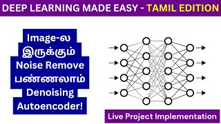


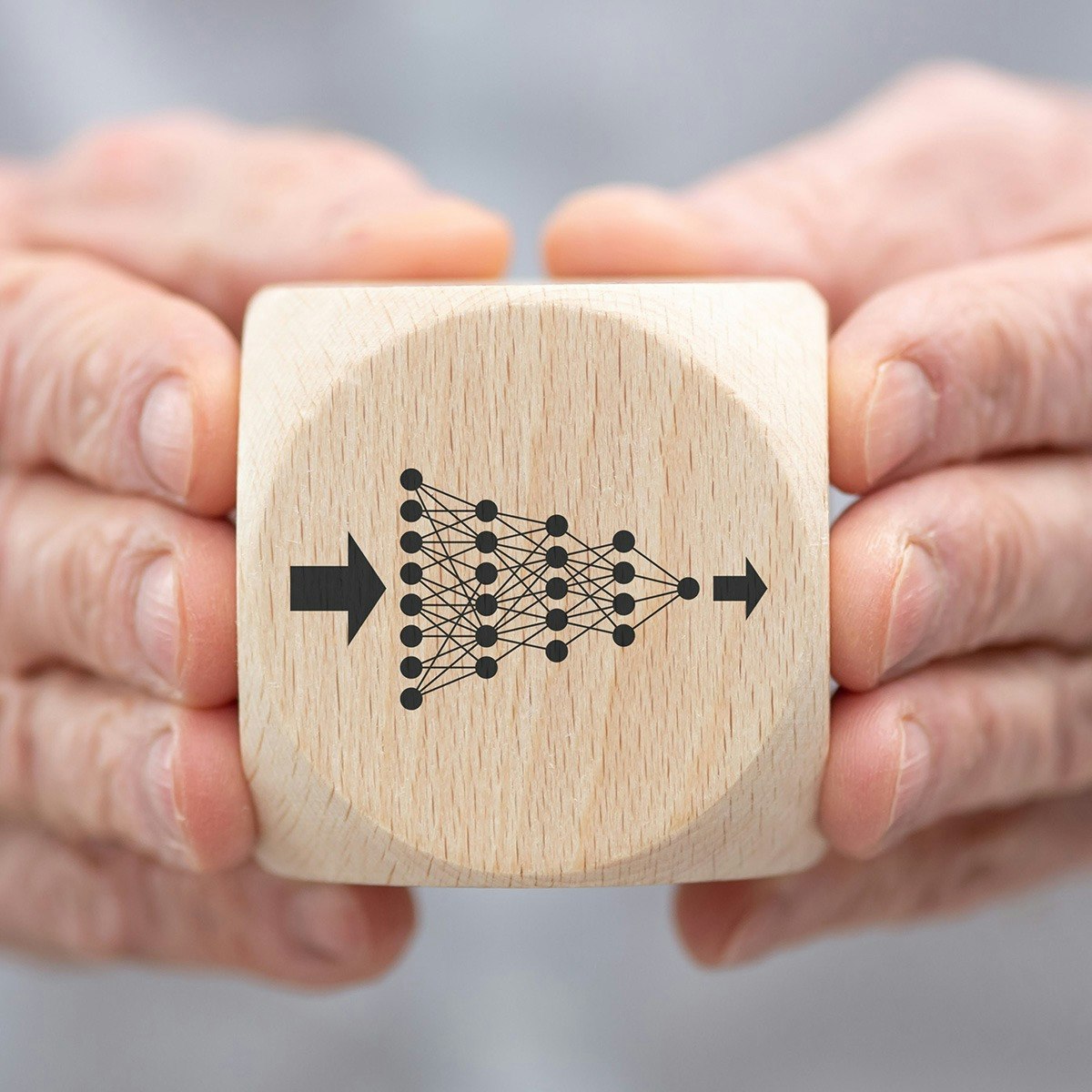


Related Reads
📰
📰
📰
📰
How to Choose the Best Deep Learning Model for Medical Imaging
Medium · Deep Learning
Another Way to Read Neural Geometry
Medium · Data Science
Another Way to Read Neural Geometry
Medium · Deep Learning
Building My First Neural Network From Scratch with PyTorch: A Journey on the Dry Bean Dataset
Medium · Deep Learning
🎓
Tutor Explanation
 DeepCamp AI