Causal Effects via Propensity Scores | Introduction & Python Code
Key Takeaways
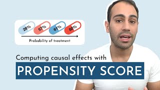
This video introduces the concept of Propensity Scores and their use in estimating causal effects from observational data, with a focus on Python implementation using logistic regression and libraries such as do_y, pandas, and numpy. The video covers three methods for computing causal effects via Propensity Scores: matching, stratification, and inverse probability of treatment weighting.
Full Transcript
hey folks welcome back this is the second video in a series on causal effects in the last video we learned some theoretical Concepts that underlie causal effects however there were questions surrounding how to translate this Theory into practice in this video we will resolve these questions with a set of practical techniques for estimating causal effects these techniques are all based on something called a propensity score we will conclude the discussion with a concrete example with python code and real world data so with that let's get into the video so in the last video of this series we were talking about estimating causal effects and to estimate causal effects we need data but not all data are equal and so here I'm going to distinguish two types of ways we can obtain data so the first is data from what I'll call an observational study so an observational study insists of passively measuring data without intervention in the data generating process so as an example the causal effect of taking a pill on headache status would an observational study might look like is we passively observe a population of people with headaches some of them taking pills some of them not taking pills and just doing an analysis trying to quantify the causal effect of that pill on headache status the second type of way we can obtain data is from what I'll call an Interventional study and what this consists of is an intentional manipulation of a data generating process for a particular goal so an example of this is a randomized control trial which we talked about in the previous video so if we were interested in studying the same thing the effect of a pill on headache status what a randomized controlled trial would look like is we pick a group of people from a larger population of people with headaches we split that group into two subgroups the first of which we give all the people a pill and then the other subgroup we don't give them a pill and then we can evaluate the causal effect so like I mentioned in the previous video Interventional studies or randomized control trials or something like it is one of the most common ways to quantify causal effects but this comes at a cost it takes a lot more effort and care to collect data through a randomized control trial than it is to just passively observe natural behaviors of people so it would be very advantageous if we could compute causal effects using observational data because it is a lot easier to obtain but there's a problem here in observational studies there could be systematic differences between people that take the pill and don't take the pill that can bias your estimate so for this example where we're just passively observing people with headaches not controlling who takes the pill and who doesn't take the pill there could be a variable that we might not be measuring such as age that could be a confounder because someone's age could drive their behavior to take a pill like kids probably won't be taking pills because their parents won't let them adults might be more likely to take pills than kids because they don't need permission from anyone to take a Tylenol and then that could also affect headache status kids might be less prone to get headaches than adults and so this introduces a systematic difference that can bias our causal effect estimate so one solution to this problem is the propensity score and so a propensity score aims to solve this problem of systematic differences by estimating the probability a subject receives a treatment based on other characteristics so essentially what we do is we include additional variables to our treatment and outcomes so our treatment variable could be takes pill or not our outcome could be headache status and then we can collect other variables that might influence treatment status or headache status such as age income sex or some other variables and so a common way of computing the propensities score is a two-step process first we train a logistic regression model so what that consists of is taking your covariates basically any variable that's not your treatment or outcome and so let's say here we have age income and sex and then we set as our Target variable the treatment status so in other words we're using the covariates to predict treatment status and logistic regression is just a way to connect a set of predictors to a binary Target once we get the logistic regression model the next step is to use it to generate the propensity score so what this might look like is we take a subject with a set of covariates here we have age income and sex we pass them into the logistic regression model that we just developed and then out comes a probability of treatment or in other words a propensity score and so now we can do this for all our subjects and we have a propensity score for every single subject in our data set with a propensity score for every subject in our observational data set we can use the propensity score in different ways to help estimate unbiased causal effects and here I'll be talking about three different propensity score based methods for doing this and so these methods are matching stratification and inverse probability of treatment waiting okay so starting with matching in the simplest case what matching consists of is creating treated untreated pairs with similar propensity scores what this might look like is we have an observational data set so we've just passively observed People's Natural behaviors when they have a headache let's say five people took a pill seven people didn't take the pill and we have propensity scores for each of these subjects and notice that there are people that actually took the pill that have a relatively low probability of treatment and conversely there are people that didn't take the pill that have a relatively high probability of treatment so this is good because it helps us in doing the matching process so one way we can do this is called one to one unmatching without replacement say we pick this subject with a 93 percent probability of treatment and what we do is match this subject to a subject in the untreated population with the most similar propensity score so we can just look at all these subjects we see 73 is the closest to 93 out of all these participants and we just match these two together and then we can take this subject with the 80 propensity score and then we do the same process excluding this participant here with 73 and then we pick this participant with a 57 percent pick the closest one in the untreated population so on and so forth so now we have a so-called matched sample and this is reminiscent of what we might see in a randomized control trial we have two groups of equal size one group took a treatment the other group didn't take the treatment so with this match sample we can compute the average treatment effect just like we did in the previous video so conceive of probably there are two ways we could go about this the first way ate stands for average treatment effect defined in the previous video e is the expectation value which is essentially an average Y is denoting the outcome variable one is indicating a treatment status of one meaning they took the pill zero is indicating a treatment status of zero meaning they didn't take the pill and I is just indexing these pairs in the Matched sample so kind of walking through this I equals one let's say it corresponds to this matched pair so this person corresponds to this term and then this person corresponds to this term we take their difference then we look at this pair we take the difference in their outcomes then we look at the next pair look at the difference in their outcomes and so on and so forth and now we'll have five values corresponding to the difference in outcomes for each of these pairs and then we can just take their average and then that'll give us an average treatment effect alternatively we can use the Expression we had for a randomized control trial so that's what RCT means here so this is is the average treatment effect in a randomized controlled trial so it's just slightly different instead of taking five differences and Computing the average here we will look at all the participants in the treated population look at their outcome and compute the average then we look at the outcome for the untreated population and then we take their difference so these are two alternative ways we can compute an average treatment effect with a matched sample so here there are a lot of details that I glossed over and I don't want to spend too much time on it I'll just refer you to this nice paper by Austin where he dives into details on optimizing the Matched sample basically how we match the took pill population with the didn't take pill population and then also Alternatives and matching so here we did one-to-one matching but you can also do one-to-many matching so essentially there what you're doing is instead of pairing each individual in the treated population with one subject in the untreated population you can match many untreated subjects to a single treated subject and this is all in the paper for anyone who is interested so we'll move on to stratification so in stratification we split subjects into groups with similar propensity scores so again let's say we have our observational data set five people took the pill seven people didn't take the pill and then what we do is what is called rank ordering so basically we order the subjects from lowest to highest propensity score so this is like what you do in elementary school math take the subjects from smallest propensity score to largest propensity score and then what we can do is split them into groups so here we split the subjects into four equal sized groups and then what we can do is compute the average treatment effect in each of these groups don't worry too much about the notation here so G is just indexing each group so we can have group one group two group three group four and then p is just indexing the people that took the pill and is indexing the people that didn't take the pill and we can compute the average treatment effect for each group like this so looking at this term this is the expectation value the average outcome for the people that took the pill let's say in group one so let's say G is equal to one and then this for g equals one we look at the average outcome for the people that didn't take the pill and since it's just one person we just look at this one person's outcome and then we take the difference and then we have the average treatment effect for group one we can do the same thing for group two then for group three group four so we have four average treatment effects and then we can go a step further and compute the average of these four averages and get an overall average treatment effect all right the last method I'll talk about is inverse probability of treatment waiting or iptw for short and the first two methods were kind of similar where we were clumping together people with similar propensity scores and comparing average outcomes between people that took the pill and didn't but in iptw we do things a little differently so here instead we use the propensity score to derive five weights from which the average treatment effect can be computed directly so what this might look like is we have our same observational data set five people take the pill seven people didn't take the pill we have propensity scores for all 12 of these individuals then we can convert these propensity scores into weights and so how we Define the weight will depend on whether the subject hooked the pill or didn't take the pill if they took the pill we just do one divided by the propensity score so 1 divided by 0.23 is about 4.35 1 over 0.93 is about 1.08 so on and so forth but if they didn't take the pill we do one divided by 1 minus their propensity score and then we can get weights for each of the subjects okay and then the next step is we use these weights to aggregate the outcomes for the treated and untreated populations so we weight each outcome so p is indexing again the people that took the pill we do this for every subject in the treated population we multi put these together we add them all up and then we divide by n which is the total number of subjects so in this case it would be 12 and then that gives us the aggregated outcome for the treated population then we do the same exact thing for the untreated population which will give us the aggregated outcome for the untreated and then we can use these values to estimate our average treatment effect so here we can just simply take the difference between the aggregated outcome of the treatment with the aggregated outcome of the untreated now we're going to do a concrete example in Python so here we'll compute the average treatment effect of going to grad school on income and for those of you keeping up with the causality videos I've been putting up this example will be very similar to what we saw in the causal inference video this code and much more is available at the GitHub which I will link in the description below so first we import our libraries so we have pickled just to import our data do y is going to help us do the causal effect estimation and then we have numpy to just do some math then we load in the data we have this pickle file which is a pandas data frame also available at the GitHub repository and then this data comes from the UCI machine learning data repository which I will link in the description as well okay next we Define the causal model so this isn't really necessary for the propensity score based techniques but this is a standard procedure in the do y Library we'll get a better sense of why the library is set up in this way in future videos of this series but for now we can just view this as picking out or labeling which variables in our data set are the treatments the outcomes and the covariance so our treatment is the variable has graduate degree which is a Boolean variable indicating whether the subject went to grad school our outcome variable is greater than 50k indicating whether the participant makes more than fifty thousand dollars or not and then we have the common causes which here we can just view as the covariates and we just have H as the single covariant and so what this causal model looks like is this this is identical to what we saw in the causal inference video and then we can compute the causal effects using these three different propensity score based methods so here we're just creating the S demand which isn't so important here but we will see why this is very important in future videos of this series and then I create a list of the names of each of the propensity score based methods so we have matching stratification and waiting then I initialize two data structures a dictionary and a list to store the causal estimates for each of these approaches and then we just compute each causal effect in a for Loop so just one by one for each of these elements in this list we're just going through and Computing the causal estimate and then storing those in both the dictionary and the list that I created earlier so the result of all this is for matching we had an average treatment effect of 0.136 for stratification we had 0.25 and for inverse probability of treatment weighting we had an average treatment effect of 0.331 so it's interesting to see that all three methods even though they're all using the same data give different causal estimates so one thing we can do is just aggregate these and take their average and so the average of all three methods is 0.24 for those of you who recalled the causal inference video where we did an identical analysis but there instead of using propensity score based methods we use something called a meta learner and we got a similar result so they're the average treatment effect was 0.2 and here we have 0.24 so very similar so how we can interpret this result is going to grad school will increase the probability someone makes more than fifty thousand dollars a year by 24 okay so before we jump with joy and say that we can compute causal effects from any observational data set I would share a word of caution so the whole point that people go through the trouble of randomized control trial is that they can handle both measured and unmeasured confounders through the randomization process you can mitigate systematic differences between your treated and untreated populations but with these propensity score based methods we can only hope to handle measured confounders in the example that we just ran through we had only a single measured confounder which was age but there are conceivably other variables that could impact both someone's probability of going to grad school and someone's probability of making more than fifty thousand dollars a year things like parental income or field of study or work ethic and so on and so forth so these propensity score based methods won't be able to account for other confounders that are not included in the propensity score model and so this may not be such a big deal when you know what you need to measure and you have the ability to measure it but the situations where you know what you need to measure but it's very tricky key to measure so for example let's say we're considering work ethic as a confounder to both someone's probability of going to grad school and someone's probability of making more than fifty thousand dollars a year it could be challenging to quantify work ethic and measuring that for each of your subjects so that brings up the problem of unmeasured confounders and so in the next video of this series we will see what we can do about unmeasured confounders okay and lastly there is a Blog associated with this video linked here and I'll also link it in the description there are some details in the blog that I didn't discuss here so for those interested feel free to check that out and if you enjoyed this video please consider liking subscribing or sharing the content if you have any questions please share those in the comments section below I definitely learned a lot from the feedback I get in the comments section and as always thanks for your time and thanks for watching
Original Description
🤝 Work with me: https://aibuilder.academy/yt/dm-BWjyYQpw
🚀 Ship AI apps in weeks, not months: https://aibuilder.academy/courses/yt/dm-BWjyYQpw
This is the 2nd video in a series on causal effects. Here I introduce the Propensity Score and discuss 3 ways we can use it to compute causal effects from observational data. At the end, I share a concrete example with code of what using these methods might look like in practice.
👉 Series Playlist: https://www.youtube.com/playlist?list=PLz-ep5RbHosVVTz9HEzpI4d6xpWsc8rOa
📰 Read more: https://medium.com/towards-data-science/propensity-score-5c29c480130c?sk=45f0ec6803eba962c0d2d0162185741d
💻 Example Code: https://github.com/ShawhinT/YouTube-Blog/tree/main/causality/propensity_score
Resources:
- An Introduction to Propensity Score Methods for Reducing the Effects of Confounding in Observational Studies by Peter C. Austin
- Data from UCI MLR: https://archive.ics.uci.edu/ml/datasets/census+income
Introduction - 0:00
Observational vs Interventional Studies - 0:32
Propensity Score - 3:25
3 Propensity Score-based Methods - 4:56
1) Matching - 5:18
2) Stratification - 9:07
3) Inverse Probability of Treatment Weighting - 10:37
Example: ATE of Grad on Income - 12:29
Word of Caution - 15:46
Watch on YouTube ↗
(saves to browser)
Sign in to unlock AI tutor explanation · ⚡30
Playlist
Uploads from Shaw Talebi · Shaw Talebi · 22 of 60
1
 2
2
 3
3
 4
4
 5
5
 6
6
 7
7
 8
8
 9
9
 10
10
 11
11
 12
12
 13
13
 14
14
 15
15
 16
16
 17
17
 18
18
 19
19
 20
20
 21
21
 ▶
▶
 23
23
 24
24
 25
25
 26
26
 27
27
 28
28
 29
29
 30
30
 31
31
 32
32
 33
33
 34
34
 35
35
 36
36
 37
37
 38
38
 39
39
 40
40
 41
41
 42
42
 43
43
 44
44
 45
45
 46
46
 47
47
 48
48
 49
49
 50
50
 51
51
 52
52
 53
53
 54
54
 55
55
 56
56
 57
57
 58
58
 59
59
 60
60
biometricDashboard2 DEMO
Shaw Talebi
biometricDahboard3 DEMO
Shaw Talebi
Time Series, Signals, & the Fourier Transform | Introduction
Shaw Talebi
The Fast Fourier Transform | How does it (actually) work?
Shaw Talebi
The Wavelet Transform | Introduction & Example Code
Shaw Talebi
Principal Component Analysis (PCA) | Introduction & Example (Python) Code
Shaw Talebi
Independent Component Analysis (ICA) | EEG Analysis Example Code
Shaw Talebi
Kmeans-based Blink Detecter DEMO
Shaw Talebi
Shit Happens, Stay Solution Oriented
Shaw Talebi
Why Conflict Is Good & How You Can Use It
Shaw Talebi
Causality: An Introduction | How (naive) statistics can fail us
Shaw Talebi
Causal Inference | Answering causal questions
Shaw Talebi
Causal Discovery | Inferring causality from observational data
Shaw Talebi
How to Be Antifragile | 7 Practical Tips
Shaw Talebi
Multi-kills: How to Do More With Less (no, not by multi-tasking)
Shaw Talebi
Topological Data Analysis (TDA) | An introduction
Shaw Talebi
The Mapper Algorithm | Overview & Python Example Code
Shaw Talebi
Persistent Homology | Introduction & Python Example Code
Shaw Talebi
What Is Data Science & How To Start? | A Beginner's Guide
Shaw Talebi
How to do MORE with LESS - multikills
Shaw Talebi
Causal Effects | An introduction
Shaw Talebi
Causal Effects via Propensity Scores | Introduction & Python Code
Shaw Talebi
Causal Effects via the Do-operator | Overview & Example
Shaw Talebi
Causal Effects via DAGs | How to Handle Unobserved Confounders
Shaw Talebi
Smoothing Crypto Time Series with Wavelets | Real-world Data Project
Shaw Talebi
Causal Effects via Regression w/ Python Code
Shaw Talebi
5 Reasons Why Every Data Scientist Should Consider Freelancing
Shaw Talebi
An Introduction to Decision Trees | Gini Impurity & Python Code
Shaw Talebi
10 Decision Trees are Better Than 1 | Random Forest & AdaBoost
Shaw Talebi
Dimensionality Reduction & Segmentation with Decision Trees | Python Code
Shaw Talebi
How to Make a Data Science Portfolio With GitHub Pages (2025)
Shaw Talebi
My $100,000+ Data Science Resume (what got me hired)
Shaw Talebi
How to Create a Custom Email Signature in Gmail (2025)
Shaw Talebi
I Spent $675.92 Talking to Top Data Scientists on Upwork—Here’s what I learned
Shaw Talebi
Lessons from Spending $675.92 to Talk to Top Data Scientists on Upwork #freelance #datascience
Shaw Talebi
A Practical Introduction to Large Language Models (LLMs)
Shaw Talebi
The OpenAI (Python) API | Introduction & Example Code
Shaw Talebi
The Hugging Face Transformers Library | Example Code + Chatbot UI with Gradio
Shaw Talebi
Why I Quit My $150,000 Data Science Job
Shaw Talebi
Prompt Engineering: How to Trick AI into Solving Your Problems
Shaw Talebi
The REALITY of entrepreneurship. #entrepreneurship #startup #smallbusiness
Shaw Talebi
Fine-tuning Large Language Models (LLMs) | w/ Example Code
Shaw Talebi
How to Build an LLM from Scratch | An Overview
Shaw Talebi
I Have 90 Days to Make $10k/mo—Here's my plan
Shaw Talebi
I Spent $716.46 Talking to Data Scientists on Upwork—Here’s what I learned.
Shaw Talebi
Pareto, Power Laws, and Fat Tails
Shaw Talebi
Do NOT become an entrepreneur #entrepreneurship
Shaw Talebi
Detecting Power Laws in Real-world Data | w/ Python Code
Shaw Talebi
How I’d learn data analytics (if I had to start over in 2024) #dataanalytics
Shaw Talebi
4 Ways to Measure Fat Tails with Python (+ Example Code)
Shaw Talebi
Fine-tuning EXPLAINED in 40 sec #generativeai
Shaw Talebi
How Much YouTube Paid Me in My First 6 Months of Monetization (as a Data Science Creator)
Shaw Talebi
5 Questions Every Data Scientist Should Hardcode into Their Brain
Shaw Talebi
AI for Business: A (non-technical) introduction
Shaw Talebi
LLMs EXPLAINED in 60 seconds #ai
Shaw Talebi
3 Ways to Make a Custom AI Assistant | RAG, Tools, & Fine-tuning
Shaw Talebi
What is #ai? — Simply Explained
Shaw Talebi
QLoRA—How to Fine-tune an LLM on a Single GPU (w/ Python Code)
Shaw Talebi
How to Improve LLMs with RAG (Overview + Python Code)
Shaw Talebi
Text Embeddings, Classification, and Semantic Search (w/ Python Code)
Shaw Talebi
More on: LLM Foundations
View skill →


![Run Any AI LOCALLY for FREE Forever! [100% Beginner Tutorial]](https://i.ytimg.com/vi/8GFPZRgtEn8/mqdefault.jpg)


Related Reads
📰
📰
📰
📰
How I Built a Free Online Image & PDF Processing Platform with Vue 3 + FastAPI
Dev.to · IAMUU
I Built a Free AI-Powered YouTube SEO Toolkit With Zero Budget. Here’s What Actually Happened.
Medium · Startup
How to Create a Second Version of Yourself Inside Obsidian Using AI (Step-by-Step Guide)
Medium · ChatGPT
How to prepare for Spain civil service TIC exam using AI in 2026
Dev.to · David García
🎓
Tutor Explanation
